JING Hai-xiao （荆海晓）， LIU Chang-gen （刘长根）， TAO Jian-hua （陶建华）

Department of Mechanics， Tianjin University， Tianjin 300350， China， E-mail: jinghx@tju.edu.cn

An extended form of Boussinesq-type equations for nonlinear water waves*

JING Hai-xiao （荆海晓）， LIU Chang-gen （刘长根）， TAO Jian-hua （陶建华）

Department of Mechanics， Tianjin University， Tianjin 300350， China， E-mail: jinghx@tju.edu.cn

2015，27（5）:696-707

An extended form of Boussinesq-type equations with improved nonlinearity is presented for the water wave propagation and transformation in coastal areas. To improve the nonlinearity of lower order Boussinesq-type equations，without including higher order derivative terms， an extended form of Boussinesq-type equations is derived by a generalized method. The Stokes-type analysis of the extended equations shows that the accuracy of the second order and third order nonlinear characteristics is improved greatly. The numerical test is also carried out to investigate the practical performance of the new equations under different wave conditions. Better agreement with experimental data is found in the regions of strong nonlinear wave-wave interaction and harmonic generation.

Boussinesq-type equations， nonlinearity， Stokes-type analysis， harmonic generation

Introduction

Boussinesq-type equations can be used to study the water wave refraction， diffraction， the wave-wave interaction and the harmonic generation and so on. It is a popular choice for simulating the water wave propagation and transformation in the near-shore areas. In the derivation of the classical Boussinesq equations，two fundamental assumptions are made. One is the vertical distribution of the horizontal velocities， which is mostly approximated by the Taylor expansion. Another is the weak dispersion and the weak nonlinearity，ε=O（µ2）≪O（1）， whereµis the ratio of the depth h to the wave lengthL， andεis the ratio of the amplitudeAto the depthh. Weak nonlinearity of the classical Boussinesq equations is a critical limitation when the equations are used to simulate the water wave propagation in a surf zone.

In order to improve the nonlinear characteristics of Boussinesq-type equations， several methods based on the two assumptions were developed. First， the nonlinearity of Boussinesq-type equations is improved by using more accurate approximations for the vertical distribution of the horizontal velocities. For example，higher order terms in the Taylor expansion are included in the derivation， such as by Gobbi et al.［1］. This is a straightforward idea to improve the nonlinear characteristics of Boussinesq-type equations. The Padé approximation is typically more accurate than the Taylor approximation. This is also used when the vertical distribution of the horizontal velocities is approximated，as used by Agnon et al.［2］， Madsen et al.［3］and others. Also， the multilayer method is used to improve the accuracy of the approximations， and then to improve the nonlinearity， such as by Lynett and Liu［4］. Secondly， various relations ofεandµare assumed， such aswas used by Zhang and Tao［5］andwere used by Wei et al.［6］. Besides， higher order nonlinear terms in the equations can be modified by introducing extra terms with free parameters， such as by Schäffer and Madsen［7］， Zhang and Tao［5］， Fang et al.［8］. Moreover， Kennedy et al.［9］presented a set of Boussinesq-type equations with an improved nonlinear performance by extending the reference velocity used in the governing equations to vary with time.

For the first type， the nonlinear properties of the equations are improved greatly by improving the accuracy of the approximations for the vertical distribution of the horizontal velocities. These methods lead to Boussinesq-type equations with higher order derivative terms or more governing equations than theprevious ones. While the second method improves the nonlinear characteristics by assuming different relations betweenµandε， such as ε=O（µ）or ε=O（1）. By doing this， more nonlinear terms are included in the governing equations， and the highest order of derivative terms is still three. In the method by Kennedy et al.［9］， more free parameters determined by matching with the Stokes solutions for nonlinearity were introduced in the governing equations.

The Boussinesq-type equations with better accuracy for the nonlinearity bring about difficulties for obtaining their numerical solutions， which means more computational efforts. This is why the lower order Boussinesq-type equations derived by Wei et al.［6］were used widely in coastal engineering. Considering these problems， many attempts were made to improve the nonlinear properties of Boussinesq-type equations and to hold the highest order of derivative terms no more than three， meanwhile no more additional equations to be involved， such as by Zhang and Tao［4］， Karambas and Memos［10］， Klopman et al.［11］，Galan et al.［12］， Fang et al.［13］and Fang et al.［8］， among others. For these purposes， a straightforward method is to further improve the properties of Boussinesq-type equations with order O（µ2）where the highest order of derivative terms is three. Fang et al.［8］presented an extension of the lower order Boussinesq-type equations obtained by Schäffer and Madsen［7］with improved nonlinearity. Meanwhile， Karambas and Memos［10］developed a new set of Boussinesq-type equations， in which all the higher order derivative terms were expressed through convolution integrals. These equations can be solved by using a simple finite difference method. But the numerical integration of a convolution integral is required. Klopman et al.［11］derived a new set of Boussinesq-type equations based on the variational principle. The equations contain only lower order spatial derivatives without mixed time-space derivatives. Besides， Antuono and Brocchini［14］proposed some radically-new approaches to derive Boussinesq-type equations which can be solved numerically applying hyperbolic-type solution methods and are valid for highly nonlinear waves.

This paper focuses on the improvement of nonlinearity of lower order Boussinesq-type equations. Based on the lower order Boussinesq-type equations derived by Zhang and Tao［5］under the assumption of ε=O（µ）， an extended form of lower order Boussinesq-type equations is derived. The extended equations enjoy better accuracy for the nonlinearity，and they are easy to be solved numerically.

1. Derivation of extended boussinesq-type equations

We start from the non-dimensional form of Boussinesq-type equations derived by Zhang and Tao［4］. They are as follows:

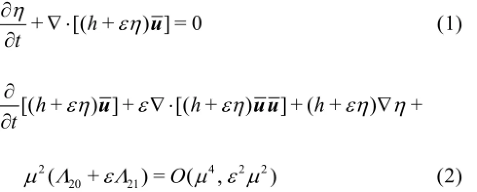
whereη andu represent the dimensionless free surface elevation and the depth averaged velocity， respectively.t is the dimensionless time， andhdenotes the dimensionless water depth.is the gradient operator. And

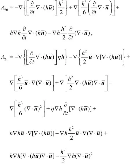
The derivation of Eqs.（1）， （2） is based on the assumption of ε=O（µ）≪O（1）. This assumption allows for stronger nonlinearity in the equations than the traditional assumption ofε=O（µ2）≪O（1）.

Next， we modify the above equations by using a generalized method of Schäffer and Madsen［7］. This method was also used by Fang et al.［8］. Two operators，and， are introduced in this method， where the free parametersα1and α2are determined to give better linear properties. In this paper， the nonlinear terms and the corresponding free parameterγare introduced in the operators， which are used to deal with nonlinearity as Schäffer andMadsen［7］did for linearity. This is similar to the method of Kennedy et al.［9］who generalized the reference elevation of Wei et al.［6］to make it vary with time. The procedure of the method is as follows:

Applying the operator αµ2（h+γεη）2∇（∇·）to1Eq.（2） yields

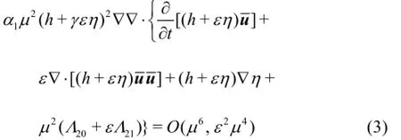
Neglecting the terms with orders higher than O（µ4）

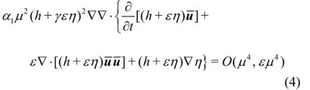
Multiplying Eq.（2） by （h+γεη）and then applying the operator［αµ2（h+γεη）∇（∇·）］， we have 2

Neglecting O（µ4）terms and higher order terms

Equation （4） and Eq.（6） are added into Eq.（2），and the final momentum equations become

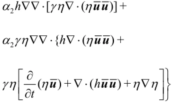
where Equation （1） and Eq.（7） are the new governing equations for the dispersive and nonlinear water wave propagation and transformation. Comparing the modified Eq.（7） with Eq.（2）， it can be seen that the additional terms are included in the modified equations. The terms with orders O（µ2）and O（εµ2）in Eq.（2） are modified， and the terms with orders O（ε2µ2）and O（ε3µ2）which represent higher order nonlinear terms are included in the new equations. Zhang and Tao［4］also presented a set of equations to improve the linear property and the equations can be obtained from the new equations by setting α2=γ=0.

2. Theoretical analysis of extended equations

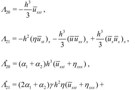
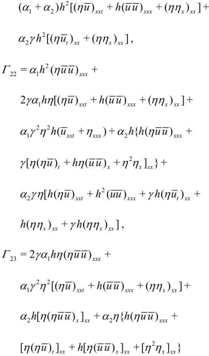
In this section， the Stokes type analysis is employed to analyze the properties （especially nonlinearities）of the extended equations described in the above section. The results are compared with the Stokes solutions and the results of the equations proposed by Zhang and Tao［5］and the equations proposed by Wei et al.［6］which are widely used in engineering applications. Then， the free parameters in the equations are determined by minimizing the combined errors. For this purpose， the 1-D formulation of the new equations with a horizontal bottom is given as:

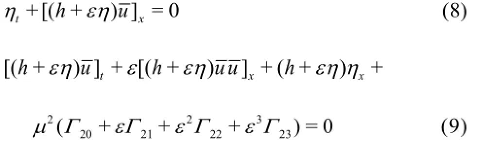
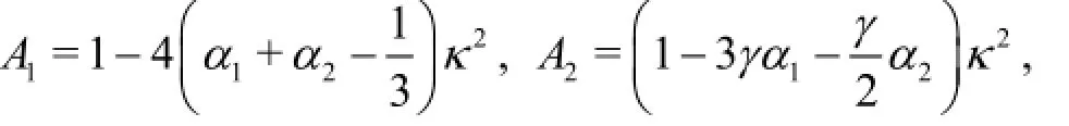
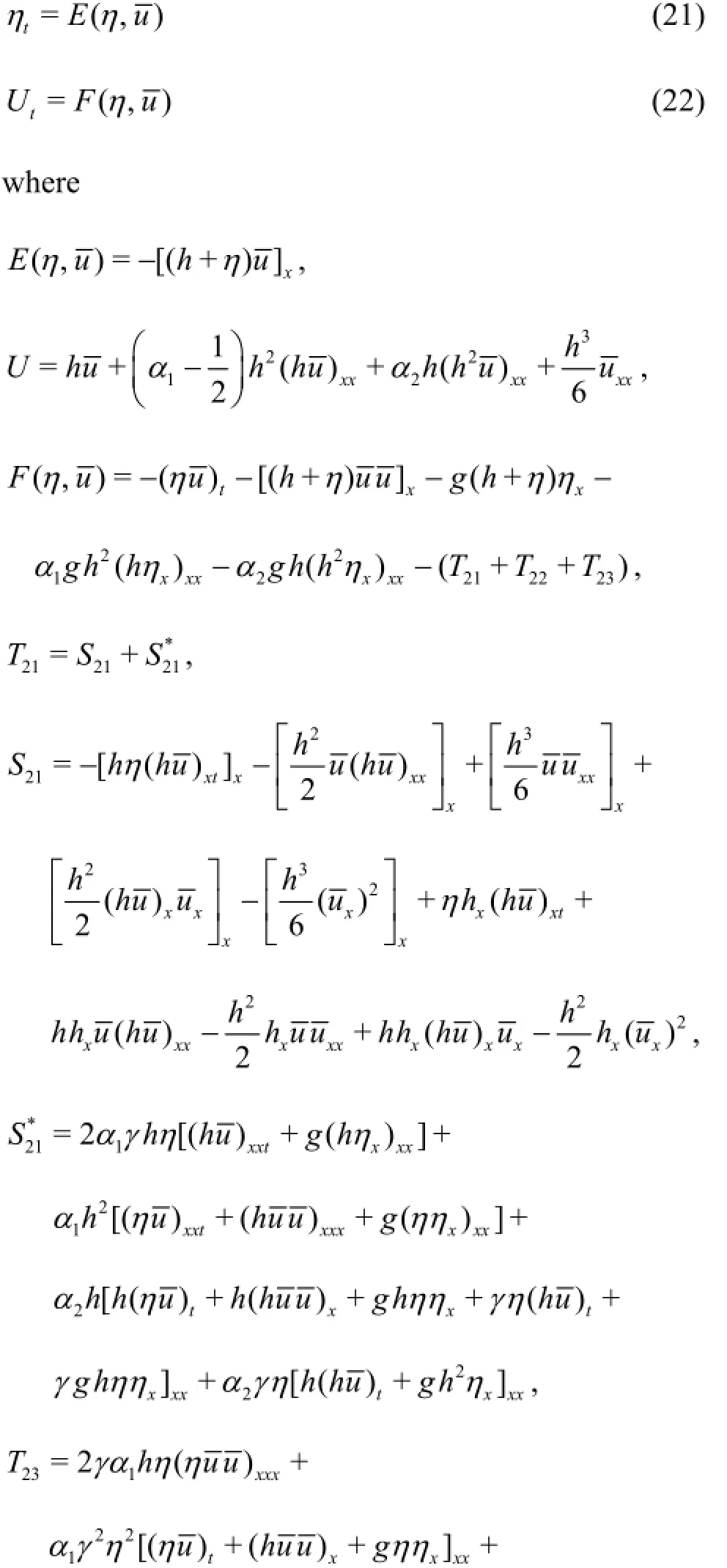
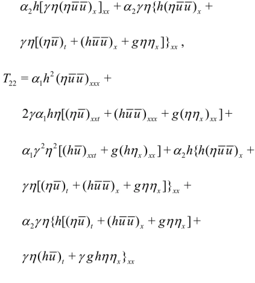
where

The following Stokes-type expansions are introduced

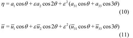
Inserting the above equations into Eq.（8） and Eq.（9）， and collecting terms ofthe governing equations for the first， second and third order problems can be obtained.

2.1 First order equations

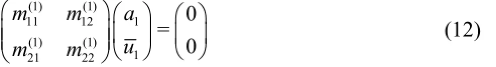
where

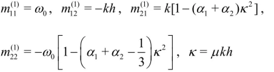
For nontrivial solutions of Eq.（12）， the determinant of coefficients should be zero. This gives the linear dispersion relation of the new equations.

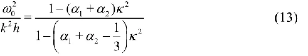
The group velocity can also be obtained from the linear dispersion relation.

where

Compared with the equations proposed by Zhang and Tao［5］and Wei et al.［6］， this set of equations enjoys the same linear accuracy.

2.2 Second order equations

For the second order， one obtains

where

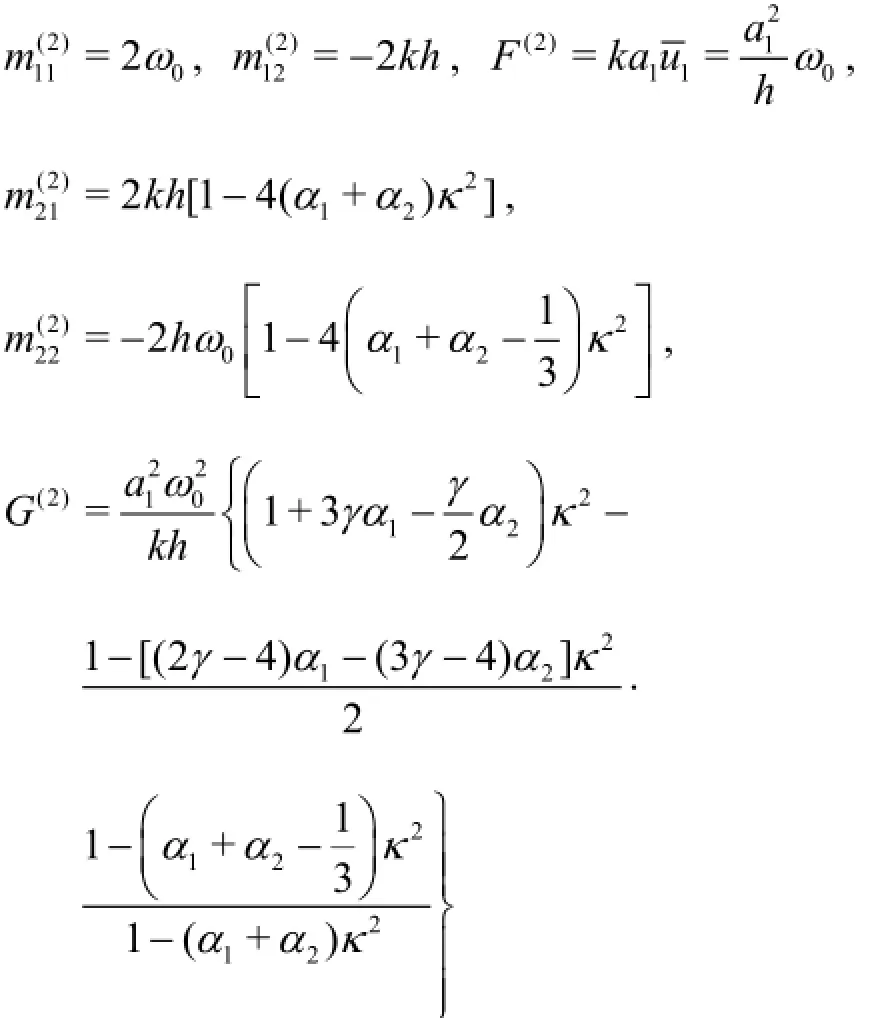
Solving the equations， we can get the second order free surface elevation

where

2.3 Third order equations

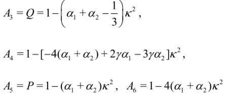
By the same method， the third order equations can be obtained as

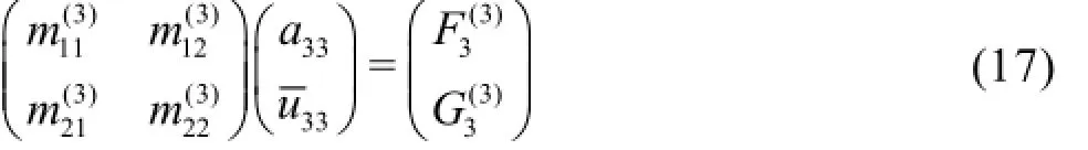
where

where

From Eq.（17） and Eq.（18）， one can solve the third order amplitude and the third order frequency dispersion.

2.4 Optimization of free parameters

In the new equations， three free parameters，α1，α2andγ， are to be determined in order to provide better linear and nonlinear properties. From the above analysis， it can be found thatα1and α2can be used for optimizing the linear properties， i.e.， the linear dispersion and the group velocity. While to optimize the nonlinear characteristics， all the three free parameters are used. To determine these free parameters， the method of minimizing the total errors in a certain range of applications will be employed. The Stokes solutions are taken as the target solutions which can be found in reference by Schäffer and Madsen［6］. Finally，α1+ α2=-0.0533is found by optimizing the linear dispersion in the range of 0＜κ＜π. This result agrees with that obtained by Fang et al.［8］. For the nonlinear properties， there are three solutions to be optimized，they are the second order free surface elevation a2，the third order free surface elevation a33and the third order amplitude dispersion ω3. Considering the fact that the second order elevation a2is more important than the third elevation a33， the combined errors of a2and ω3will be used in this study.α1=-0.0747，α2=0.0214and γ=1.75are the optimized values for the equations.

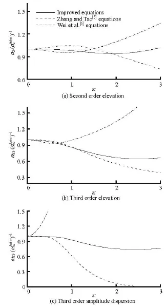
Fig.1 Comparison of （a） the second order elevation， （b） the third order elevation and （c） the third order amplitude dispersion

Finally， the results with the optimized values are shown in Fig.1. It can be seen that the accuracy of a2，a33and ω3are greatly improved comparing with both the equations proposed by Wei et al.［6］and by Zhang and Tao［5］. The accuracy of the second and third nonlinear properties of the equations is extended up to =3 κ. And it is obvious that these corrections are due to the inclusion of extra nonlinear terms.

3. Numerical test

In order to further validate the improvement of the nonlinear properties of the extended equations， a numerical test is carried out to investigate the wave propagation over a submerged bar which involves the wave-wave interaction and the harmonic generation.

3.1 Numerical scheme

The 1-D version of the extended Boussinesq equations is solved numerically. The procedure of the numerical solution follows exactly the method proposed by Wei et al.［6］and Lin and Man［15］. For the time derivative terms， the fourth order Adams predictorcorrector method is used. The first order spatial derivative terms are discretized by the fourth order central difference method. And the three-point central difference method is used for the second order spatial derivatives. This will ensure that the leading order truncation errors will not suppress the third order physical dispersion in the governing equations. To implement the numerical scheme， a new variableU is introduced and the governing equations are rewritten as follows:

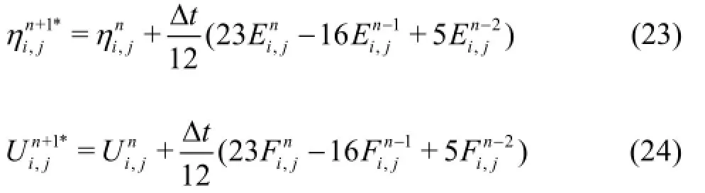
For the predictor step， the explicit third order Adams-Bashforth scheme is used and Eq.（21） and Eq.（22） become

And for the corrector step， the fourth order Adams-Moulton method is used， the results are as follows:

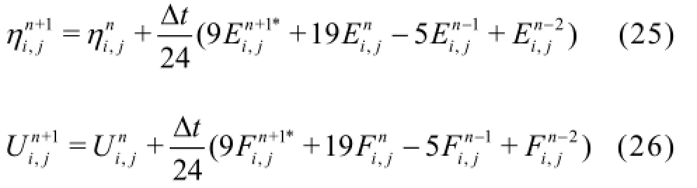
where ∆tis the time step，n denotes the current time level，n +1denotes the next time levelis the predicted elevation. The values of all terms on the right hand sides of Eq.（23） and Eq.（24） are known. So it is straightforward to obtainand. From the definition ofU ， the predicted velocitycan be obtained by solving a tri-diagonal matrix equation. After the predictor step， the predicted values ofandcan be used to calculateand. Inserting the values obtained into Eq.（25） and Eq.（26），the corrector values ofandcan be obtained. The corrector procedure will be repeated until the error is within the desired small limit.

In order to avoid the second reflection from the wave maker boundary， several methods might be adopted， such as the methods proposed by Wei et al.［16］and Zhang et al.［17］The internal wave generation method developed by Wei et al.［16］and the absorbing boundaries are employed in this paper. To implement the internal wave generation， a source term is added in Eq.（1）. The resulting continuity equation is as follows

where

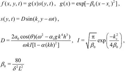
xcis the location of the center of the wave maker domain，αand α1are the coefficients related to the governing equations， and in this paper α=-0.39and α1=-0.057.kxand kyare the wave number inx andy directions.θis the angle between the wave direction and y axis. In the 1-D case in this paper，θ=0and ky=ksin（θ）is zero.L is the wave length， andδis a dimensionless number which determines the width of the wave maker domain， and δ= 0.3 is set in the following numerical test.

The method for the absorbing boundaries follows exactly the method given in Lin and Man［15］， and will not be repeated here. More details about the numerical scheme， including the stability， the tests and so on，can be found in our forthcoming paper.

3.2 Numerical results

A laboratory experiment of this test was presented by Beji and Battjes［18］. Figure 2 shows the sketch of the case， a horizontal flume of 0.4 m in water depth，a trapezoidal bar with a 1:20 front slope and a 1:10 back slope， and on the top of the bar， the water depth is 0.1 m. Seven gauges are set over the bar to measure the water surface elevations in the laboratory experiment. In this numerical study， both sides of the flume are set as the wave absorber， the width of the wave absorber boundaries is set as 3 m. The wave maker is at 8.0 m away from the left-hand side of the flume. The spatial step is ∆x=0.05mand the time step is∆t=0.01s， the total time is 40 s， the initial wave elevation and the velocity are set as zero， the optimizedfree parameters are used for the extended equations. Two cases in the experimental study are used in this paper. In one case， we have the period of 2.02 s and the amplitude of 0.01 m， which leads to kh≈0.67and a/h=0.025and in another case， we have the period of 1.01s and the amplitude of 0.0205 m， so thatkh≈1.72 and a/h=0.051. The original equations （1）， （2）and the enhanced equations （1） and （7） are used to obtain the numerical results. The results are shown in Fig.3 and Fig.4. From the results， it can be seen that better agreements are achieved for the extended equations at Gauges 5， 6 and 7 in both cases. In order to analyze the results of two numerical cases quantitatively， an index is employed here， which is as follows:

Coefficient of determination

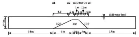
Fig.2 Sketch of wave propagation over a submerged bar. Topography and gauges where experimental data are obtained and displayed

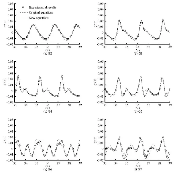
Fig.3 Comparison of results obtained by experiments， by the original equations and the new equations in the case of T =2.02s，A =0.01m（G2 to G7 denote different locations where the free surface elevations are measured）

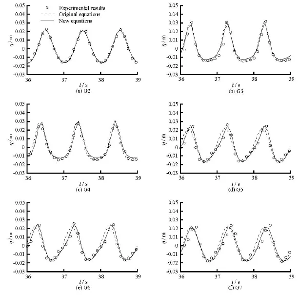
Fig.4 Comparison of results of experiments， the original equations and the new equations in the case of T =1.01s，A=0.0205m（G2 to G7 denote different locations where free surface elevations are measured）

where xiand yiare two sets of data，y is the mean value of yi，n is the number of data points. The coefficient of determination indicates how well the data points fit a line or a curve.

4. Discussions

In this section， the results of the theoretical analysis and the numerical tests in the above sections are discussed.

From the Stokes type analysis and the free parameter optimization， it can be found that， to the first order， the linear dispersion relationship and the group velocity of the extended equations are the same as those obtained by the equations proposed by Zhang and Tao［5］and Wei et al.［6］. No free parameters and higher order terms are introduced in the linear dispersion relationship and the group velocity. This is consistent with the fact that no higher order terms are introduced in the extended equations. To the second order， from Fig.1（a）， it can be seen that the free surface elevation a2of the extended equations is more accurate than the others in the range of 0＜κ＜3. The maximum error of a2for the extended equations is 5.9%，and it is 26.3% and 34.1% for the equations proposed by Zhang and Tao［5］and by Wei et al.［6］， respectively. Significant improvement is achieved for the second order elevation. For the third order elevation a33， the results are shown in Fig.1（b）. The maximum error in the range of 0＜κ＜3 is 33.3% for the extended equations. Though it is not accurate enough， a significant improvement is achieved， compared with the results by other two equations. The maximum error inthe range of 03κ＜＜ is 61.0% for the equations proposed by Zhang and Tao［5］and 99.7% for the equations proposed by Wei et al.［6］. Furthermore， as mentioned in the above section， the second order elevation2a， which has been improved obviously， is more important than the third order elevation33a. The third order amplitude dispersion3ω， which indicates the nonlinear process of the amplitude dispersion， is shown in Fig.1（c）. The error of3ωfor the equations proposed by Wei et al.［6］increases rapidly as κ increases， great errors can be found even for small values of κ. The accuracy of3ωfor the equations proposed by Zhang and Tao［5］decreases rapidly when 0.5 κ＞， whereas the errors of3ωfor the extended equations are much smaller than the two others. The maximum error in the range of 03κ＜＜ is 25.9%. The accuracy is obviously improved.

The numerical tests show that， in the first case，good agreement with experimental results is maintained at Gauges 2 to 5 for both models in Fig.3， while better performances can be found at Gauges 6 and 7 for new equations than the original equations. In order to give a quantitative measurement of the fitness between the numerical results and the experimental results， the coefficients of determination2Rat Gauges 6 and 7 are calculated. At Gauge 6，2Ris 0.726 and 0.961 for the results of the original equations and the extended equations， respectively. At Gauge 7，2Ris 0.564 for the original equations， and 0.911 for the extended equations. Great improvement can be seen at both gauges. From the FFT analysis of the experimental data， on the transmitted side （the downward slope）of the bar the second and third harmonics are released with a magnitude of the same order as the first harmonic. This requires the equations to be accurate at least to the third order. The maximum value of =khµat Gauges 2， 3， 4 and 5 is 1.55. While at Gauges 6 and 7，the values of =khµare 2.69 and 3.56， respectively. In other words， better agreement with experimental data at Gauges 2， 3， 4 and 5 requires the model to be accurate up to =1.55 kh for the first， second and third order nonlinear properties， and =kh 2.69 and 3.56 at Gauges 6 and 7 for first three order nonlinearities. From the results of the Stokes type analysis， at the range of 01.55 kh≤≤both the original and the new equations are accurate for the second and third order surface elevations. The new equations are more accurate than the original equations when =kh 2.69 and 3.56 for the second and third order nonlinearities. For the first order solution， both equations are accurate up to 3kh≈， which can be found in Zhang and Tao［5］. These can explain why the differences appear only at Gauges 6 and 7 in this case. The numerical results are consistent with the theoretical analysis.

For the second case， the incident wave is shorter and more nonlinear. For obtaining a good agreement with experimental data， the equations should involve higher order nonlinear dispersive terms. Also， from the FFT analysis， it can be found that only the first and second harmonics play important roles in the transmitted wave region， which requires that the dispersion relation and the second order elevation are more accurate. From Fig.4， the agreement with experimental data is again very good at Gauges 2 to 4 for both the original equations and the extended equations. For Gauges 5 to 7， the results of the extended equations agree better with the experimental data than those of the original equations. This indicates that the extended equations have better nonlinear dispersive properties，which are important for simulation of waves with higher nonlinearity. To give quantitative indicators for the results at Gauges 5， 6 and 7， the coefficients of determination are calculated. The values are 0.717，0.671， 0.811 for the original equations and 0.777，0.932， 0.903 for the extended equations at Gauges 5， 6 and 7， respectively. The improvement of the fitness with experimental results is obvious as well. Furthermore， the maximum value of =khµat Gauges 2， 3，4 is 2.56， and at Gauges 5， 6 and 7 the values of =µ kh are 2.86， 4.74 and 6.31， respectively. From the results of the Stokes type analysis， to the second order，both the original and the new equations are accurate when 02kh≤≤， and the new equations are more accurate than the original ones when 2kh＞. This is the reason why the differences appear only at Gauges 5， 6 and 7. Also， for the second order solution，=kh 4.74 and 6.31 are beyond the range of accuracy for both equations， this is why the results in the second case are less attractive than those in the first case.

5. Conclusion

To simulate the higher nonlinear water waves with less computer resources， the methods developed for the improvement of nonlinear characteristics of Boussinesq-type equations are reviewed in this paper. Based on the two assumptions in deriving the equations， there are mainly two methods that can improve the accuracy of the Boussinesq-type equations. The first method is to use higher accurate approximations for the vertical distribution of the horizontal velocities. Another is to assume different relations ofεandµ. Based on the Boussinesq-type equations derived by Zhang and Tao［5］under the assumption of =ε（）（1）OOµ≪and with the accuracy up to2（）Oµ， an extended form of lower order Boussinesq-type equations with improved nonlinearities is derived by the generalized method of Schäffer and Madsen［7］. Inorder to test the properties of the extended equations，the Stokes type analysis is employed and the linear dispersion， the group velocity， the second order nonlinearity and the third order nonlinearity are derived. The results are compared with the Stokes solutions and those of equations proposed by Zhang and Tao［5］and Wei et al.［6］. It is shown that the extended equations have better accuracy than the others. Furthermore， in order to test the practical performance of the new equations， a numerical test for the water wave propagation and transformation over a submerged bar is carried out. Two sets of incident waves are used in the tests. Finally， compared with the results of the original equations， the results of the extended equations show better agreement with the experimental ones in the region where high nonlinear wave-wave interactions occur. Therefore， both the theoretical and numerical analysis show that the extended equations have better nonlinear characteristics.

References

［1］ GOBBI M. F.， KIRBY J. T. and WEI G. A fully nonlinear Boussinesq model for surface waves. Part 2. Extension to O（kh）4［J］. Journal of Fluid Mechanics， 2000， 405: 181-210.

［2］ AGNON Y.， MADSEN P. A. and SCHAFFER H. A. A new approach to high-order Boussinesq models［J］. Journal of Fluid Mechanics， 1999， 399: 319-333.

［3］ MADSEN P. A.， BINGHAM H. and LIU H. A new Boussinesq method for fully nonlinear waves from shallow to deep water［J］. Journal of Fluid Mechanics， 2002， 462: 1-30.

［4］ LYNETT P.， LIU P. L. F. A two-layer approach to wave modelling［J］. Proceedings of the Royal Society of London. Series A: Mathematical， Physical and Engineering Sciences， 2004， 460（2049）: 2637-2669.

［5］ ZHANG Dian-xin， TAO Jian-hua. A Boussinesq model with alleviated nonlinearity and dispersion［J］. Applied Mathematics and Mechanics （English Edition）， 2008， 29（7）: 897-908.

［6］ WEI G.， KIRBY J. T. and GRILLI S. T. et al. A fully nonlinear Boussinesq model for surface waves. Part 1. Highly nonlinear unsteady waves［J］. Journal of Fluid Mechanics， 1995， 294: 71-92.

［7］ SCHÄFFER H. A.， MADSEN P. A. Further enhancements of Boussinesq-type equations［J］. Coastal Engineering， 1995， 26（1-2）: 1-14.

［8］ FANG K.， LIU Z. and GUI Q. et al. Alternative forms of enhanced Boussinesq equations with improved nonlinearity［J］. Mathematical Problems in Engineering，2013， 2013: 1-11.

［9］ KENNEDY A. B.， KIRBY J. T. and CHEN Q. et al. Boussinesq-type equations with improved nonlinear performance［J］. Wave Motion， 2001， 33（3）: 225-243.

［10］ KARAMBAS T. V.， MEMOS C. D. Boussinesq model for weakly nonlinear fully dispersive water waves［J］. Journal of Waterway， Port， Coastal， and Ocean Engineering， 2009， 135（5）: 187-199.

［11］ KLOPMAN G.， Van GROESEN B. and DINGEMANS M. W. A variational approach to Boussinesq modelling of fully nonlinear water waves［J］. Journal of Fluid Mechanics， 2010， 657: 36-63.

［12］ GALAN A.， SIMARRO G. and ORFILA A. et al. Fully nonlinear model for water wave propagation from deep to shallow waters［J］. Journal of Waterway， Port，Coastal， and Ocean Engineering， 2012， 138（5）: 362-371.

［13］ FANG Ke-zhao， ZHANG Zhe and ZOU Zhi-li et al. Modelling of 2-D extended Boussinesq equations using a hybrid numerical scheme［J］. Journal of Hydrodynamics， 2014， 26（2）: 187-198.

［14］ ANTUONO M.， BROCCHINI M. Beyond Boussinesqtype equations: Semi-integrated models for coastal dynamics［J］. Physics of Fluids， 2013， 25（1）: 016603.

［15］ LIN P.， MAN C. A staggered-grid numerical algorithm for the extended Boussinesq equations［J］. Applied Mathematical Modelling， 2007， 31（2）: 349-368.

［16］ WEI G.， KIRBY J. T. and SINHA A. Generation of waves in Boussinesq models using a source function method［J］. Coastal Engineering， 1999， 36（4）: 271-299.

［17］ ZHANG Hong-sheng， WANG Yan and XU Chun-hui et al. Tests and applications of an approach to absorbing reflected waves towards incident boundary［J］. China Ocean Engineering， 2013， 27（6）: 703-718.

［18］ BEJI S.， BATTJES J. Experimental investigation of wave propagation over a bar［J］. Coastal Engineering，1993， 19（1）: 151-162.

10.1016/S1001-6058（15）60532-7

（February 15， 2014， Revised July 13， 2014）

* Project supported by theNational Key Technology Support Program（Grant No. 2010BAC68B04）

Biography: JING Hai-xiao （1986-）， Male， Ph. D.

LIU Chang-gen，E-mail: lchg@tju.edu.cn