YANG Feng-Chao （杨冯超）， CHEN Xiao-peng （陈效鹏）

Department of Engineering Mechanics， Northwestern Polytechnical University， Xi’an 710129， China，

E-mail: vonchaoyoung@mail.nwpu.edu.cn

Numerical simulation of two-dimensional viscous flows using combined finite element-immersed boundary method*

YANG Feng-Chao （杨冯超）， CHEN Xiao-peng （陈效鹏）

Department of Engineering Mechanics， Northwestern Polytechnical University， Xi’an 710129， China，

2015，27（5）:658-667

In this paper， a method that combines the characteristic-based split finite element method （CBS-FEM） and the direct forcing immersed boundary （IB） method is proposed for the simulation of incompressible viscous flows. The structured triangular meshes without regarding the location of the physical boundary of the body is adopted to solve the flow， and the no-slip boundary condition is imposed on the interface. In order to improve the computational efficiency， a grid stretching strategy for the background structured triangular meshes is adopted. The obtained results agree very well with the previous numerical and experimental data. The order of the numerical accuracy is shown to be between 1 and 2. Moreover， the accuracy control by adjusting the number density of the mark points purely at certain stages is explored， and a second power law is obtained. The numerical experiments for the flow around a cylinder behind a backward-facing step show that the location of the cylinder can affect the sizes and the shapes of the corner eddy and the main recirculation region. The proposed method can be applied further to the fluid dynamics with complex geometries， moving boundaries， fluid-structure interactions， etc..

characteristic-based split， immersed boundary （IB） method， incompressible flow， no-slip condition， stretching grid

Introduction

In the computational fluid dynamics， the discretization of the computational domain， normally with a body-fitted procedure， is one of the most important procedures， which might be complicated and time consuming. In addition， a bad discretization reduces the simulation efficiency or even makes the calculation invalid. One of the alternative approaches is the immersed boundary （IB） method， which was first put forward by Peskin［1］in the simulation of flow around the flexible leaflet of a human heart. Numerous further improvements have been proposed since then. It was widely applied to handle various types of fluid dynamic problems， such as those related with the biological fluid mechanics［1］， the fluid-structure interaction［2］and the multiphase flows［3］.

The IB method is both a mathematical formulation and a numerical scheme［4］. Its primary advantages come from the fact that the procedure of the grid generation is greatly simplified. The generation of a body-conformal grid is much more cumbersome than that of a pure Cartesian one: the former usually consumes approximately 25% of the total computation time for typical complex geometries［5］. In addition， for moving boundary problems with a body-fitted grid， not only the dynamic meshes but also the procedures of projecting the solution onto the new grid are needed. Both steps can negatively impact the simplicity， the accuracy， the robustness and the computational cost of the solution procedure， especially， in cases involving a large deformation of the grid. On the other hand， the IB method uses a fixed Cartesian grid for fluids （or virtual fluids） and independent Lagrangian points to represent solid surfaces， which make it easier to handle complicated geometries. The coupling of the “solidpoints” and the flow is realized by the forcing density exerted on the fluids from the solid points. Unlike body-fitted grids， there are no boundary grid points，and therefore all grid points are treated in the same manner. It should be mentioned that， as a payment for the easiness， a higher grid resolution is required for a high Reynolds number flow simulation［6］. However， in some cases， it is worthwhile.

The numerical approaches for the IB method can be extensively classified into two major categories，the continuous forcing and the discrete forcing approaches. The force density of the continuous forcing approach［7］must satisfy certain mechanical relations（such as Hooke’s law）， and certain empirical parameters are involved. With the force density obtained， the wall boundaries are handled. At the same time， the discrete forcing approach［8］is implemented by discretizing the governing equations and using the no-slip conditions. Generally speaking， it is mainly used to handle flows around rigid walls.

For the N-S equation solver， we adopt the characteristic-based split （CBS） scheme， proposed by Zienkiewicz et al.［9］. It is very similar to the original Chorin split and also has similarities with other split schemes， widely employed in incompressible flow calculations［10］. With the introduction of the Characteristic Galerkin to the split， the scheme becomes more stable and can be used as a general approach to solve problems of both compressible and incompressible flows［11］. As the same interpolation function is employed for the velocity and pressure terms to discretize the N-S equations， the well-known Babuška-Brezzi condition is fully satisfied， and the calculation is fast and robust. Such method is applied in various disciplines［12］.

With the application of the aforementioned CBS and discrete forcing IB method， the structured triangular meshes are adopted to discretize the computational domain in this paper. The underlying idea is of twofold， the 2-D triangular meshes are convenient to be coupled with the FEM， especially， for stationary exterior boundaries， and its structurization makes it easier to handle the IB approaches. In this paper， the feasibility and the flexibility of the proposed method is examined， including the geometry setting， the accuracy control， etc..

1. Methodology

In the present paper， we combine the direct forcing IB approach with the CBS-FEM. They are described as follows.

1.1 Direct forcing IB approach

The main advantage of the IB approach is that the background grid is independent of the wall boundaries. We could consider a flow in a two-dimensional rectangle domainΩ， containing a one-dimensional closed boundaryΓ， as shown in Fig.1. The location of the boundary is expressed in the parametric form of X （s，t）for0≤s≤Land X（0，t）=X（L，t）. The parameterstracks the marker points on the boundary，and the governing equations for the system are as follows:

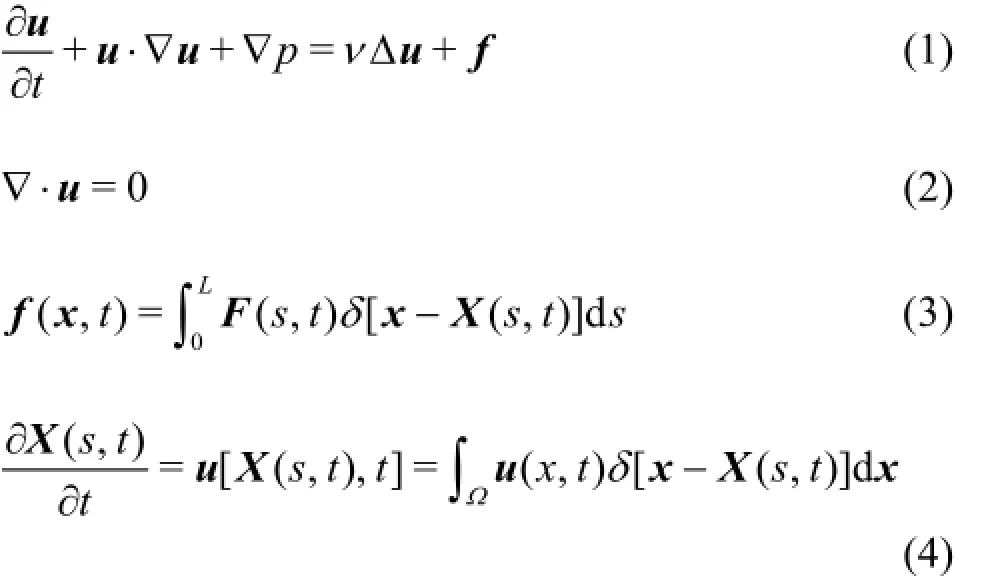
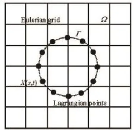
Fig.1 Configuration of immersed boundary method

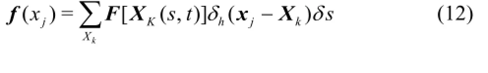
Equations （1） and （2） are the N-S equations with external force. Equation （3） describes the wall effects on the fluid by distributing the boundary force on the Lagrangian points to the Eulerian points， and Eq.（4）interpolates the velocity from the Eulerian points to the Lagrangian points. The former one （Eq.（3）） represents the interaction between the fluid and the solid force， while the latter indicates that the no-slip boundary condition is satisfied. These two equations are the essences of the IB method.

Furthermore， according to the theory of Peskin［4］，the numeric approximated δ-function in Eqs.（3） and（4） must satisfy the following criteria

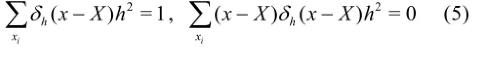
And we use the following smooth Dirac δ-function in the two-dimensional case

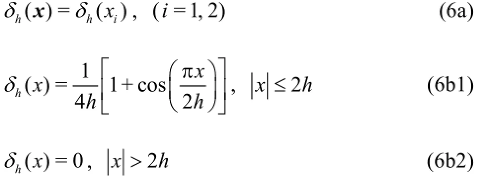
whereh is the spacing of the Cartesian grid. Other higher order moment constraints or expressions could be found in Ref.［4］.

The remaining question is how to obtain the expression of the “forcing term” corresponding to the correct wall effect. According to Eq.（1）， the hydrodynamic force at any pointxis

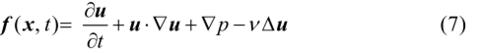
Assuming that the velocity and the pressure are known at time t=tn， then Eq.（7） can be expressed approximately in the explicit discretizing form as

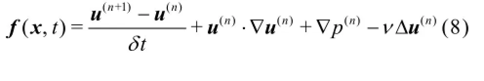
In order to satisfy the no-slip boundary conditions on the immersed boundary， we let un+1=Un+1on the boundary， i.e. the velocity u=U on the boundary x=X ， which leads to the virtual forcing density

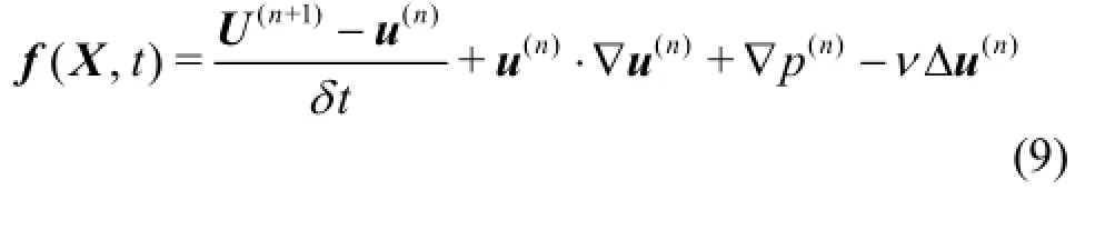
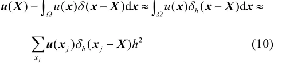
With the above equation， we come to the direct forcing approach， proposed by Fadlun［8］. The advantage of the method is that the forcing density of the immersed boundary is calculated according to the discretized N-S equations， without adding anyad hoc parameters. Since the concerneduandp are defined on the Cartesian grid and the Lagrangian points are usually off the grid， by combining with Eq.（6）， Eq.（4）can be calculated numerically as follows

The differential terms in the equation can be solved through normal discretization approaches. On the other hand， the counterforce （exerted on the Lagrangian points） could be obtained. As illustrated in Fig.2， the fluid around the Xkis forced with the density value of f（Xk）， and the corresponding counterforce on the line segmentcan be expressed as

where ε=δsh denotes the area of the considered controlled volume （grayed in Fig.2）.

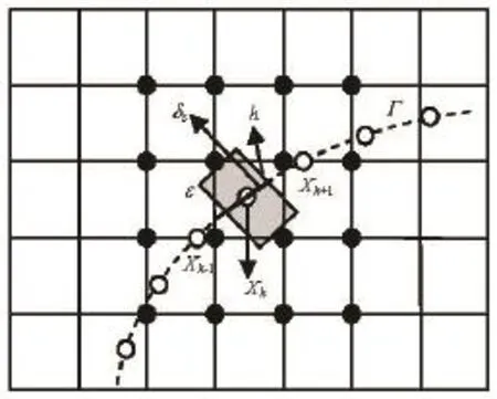
Fig.2 Calculation of the interaction forces on the immersed boundary. The horizontal and vertical lines give the Cartesian meshes. The solid discs denote the grid points influenced by the point at Xk. The dashed curve is the immersed boundary and the circles are the Lagrangian points. The thick line denotes the linear segment and the shaded rectangle is the corresponding integral areaε

We then assume that the Eulerian points （the dark points in Fig.2） in certain zone along the Lagrangian points are influenced by the wall. This influence is calculated as

Outside the zone， the wall effects are neglected， that is to say，

1.2 Characteristic-based split FEM

The derivation of the explicit CBS algorithm involves a local Taylor series expansion. The main idea of the CBS-FEM can be outlined as follows.

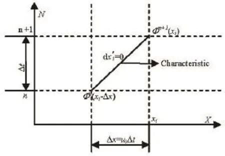
Fig.3 Characteristic in a space-time domain

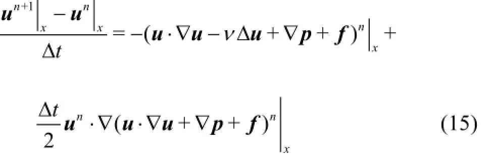
According to the characteristics Galerkin （CG）scheme［9］， we transform the coordinate by introducing a moving characteristics coordinate， as illustrated in Fig.3. From the nt hto（n+1）th levels， the incremental time interval is ∆t and the corresponding displacement of the particle is∆x. If a moving coordinate is assumed along the path of the characteristic wave with a speed ofU， the convection terms of Eq.（1） disappear （as in a Lagrangian fluid dynamics approach）. That is to say， mathematically speaking， along the characteristic line， we can transform the partial differential equation to the total differential equation （the compatibility equation）. Therefore， using the Taylor series expansion we obtain

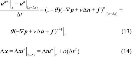
where the parameterθtakes value in the range0≤θ≤1. When θ=0， the scheme is fully explicit. And we adoptθ=0.5in this paper.

Substituting Eq.（14） into Eq.（13）， the truncated expression could be obtained through Taylor series expansion with higher-order terms neglected

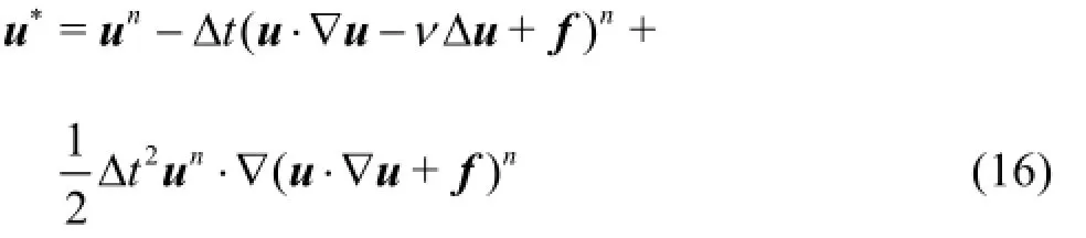
To couple the continuous and momentum equations， we introduce two-step prediction-correction procedures for the CBS algorithm. In the first step， the pressure term in the momentum equation will be dropped and an intermediate velocity field will be calculated. In the second step， the intermediate velocities will be corrected. The prediction-correction procedure is widely used in finite volume procedures or finite different schemes， with two advantages. The first is that without the pressure terms， each component of the momentum equation is similar to that of a convectiondiffusion equation and the CG procedure can be readily applied. The second advantage is that with the pressure term removed from the momentum equation， the pressure stability is enhanced and the arbitrary interpolation functions may be used for both velocity and pressure. In other words， the well-known Babuška-Brezzi condition is satisfied. It is clear that the governing equations can be solved after the temporal and spatial discretizations in the following steps:

Step 1: The intermediate velocity， the auxiliary variable， is introduced as

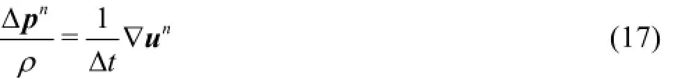
Step 2: The pressure calculation， where the Poisson equation is solved with a conjugate gradient solver

Step 3: The velocity correction

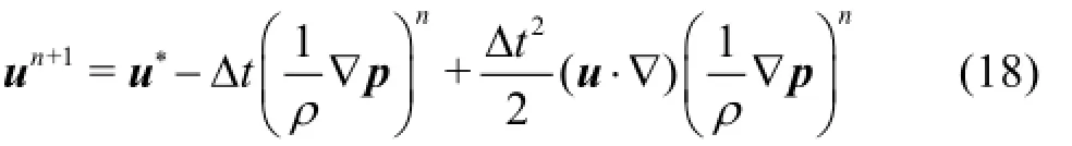
The higher-order terms in the above equations may be neglected as they have very small influence on the related velocity and pressure.

Finally， the finite element-immersed boundary method is used as follows:

（1） Obtain the forcing density by the velocity deviation between the interpolation boundary and the physical boundary using Eqs.（7）-（12）.

（2） Solve the momentum equation without pressure terms.

（3） Calculate the pressure from the Poisson equation.

（4） Correct the velocity， and finally.

（5） Go back to step 1 for iteration， until the convergence criterion is satisfied.

2. Results and discussions

To verify the flexibility and the robustness of the present approach in solving the incompressible N-S equations， three typical numerical simulations are carried out as the benchmarks， namely， the Poiseuille flow， the laminar boundary development and the flow around a cylinder. For the first two cases，Re=100（Reynolds number is defined as Re=UL/n， where U，L are the characteristic velocity and length， respectively）， and one of the wall condition is treated with the IB approach， and uniform meshes are adopted. While in the simulation of the flow past a circular cylinder，Re varies from 40 to 200. At last， the flow around a cylinder behind a backward facing step is simulated to show the combination of the feasibility of the IB method for complex external and internal geometries.

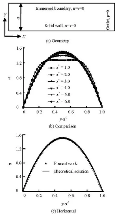
Fig.4 Flow through a 2-D rectangular channel. The continuous line represents the analytical result and the crosses denote the numerical result

2.1 Exterior boundary simulation

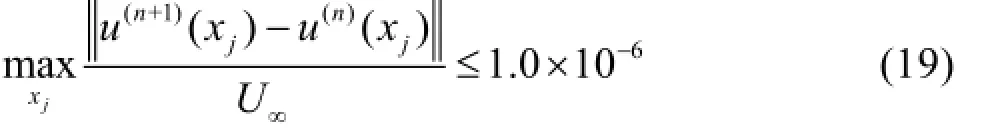
2.1.1 Poiseuille flow Figure 4（a） shows the computational domain for the Poiseuille flow. The IB approach and an exactly no-slip boundary condition are imposed on the upper and lower boundaries， respectively. The inlet Reynolds number of the flow is set to be 100 with an uniform profile， which is supposed to be a laminar flow， and the grid solution is h=0.01a . The following convergence criterion is adopted， which is also suitable for the other steady cases

The viscous boundary layer develops in the streamwise direction. Figure 4（b） shows a comparison of the velocity profiles at non-dimensional distances x∗=100vx/a2Ufrom 0 to 6. It may be observed that0the parabolic profile is reached at a distance of about 4.0， which is well consistent with the analytical solution by Schlichting［13］， who proposed that a fully developed parabolic velocity profile could be achieved after x∗=0.04Re. Figure 4（c） shows that the error of the “ultimate” velocity is less than 0.1%. And it should be noted that the consistent data are achieved near the upper and lower boundaries （y =0anda ）， where different approaches are applied as mentioned before.

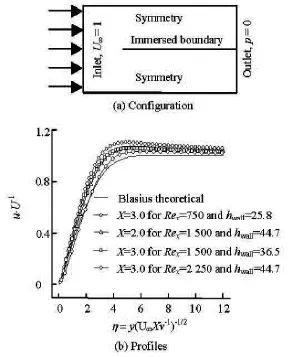
Fig.5 Flow in laminar boundary layer

2.1.2 Laminar boundary layer flow

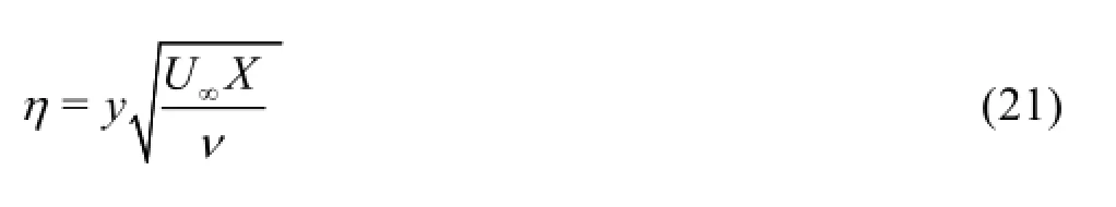
In addition， the developments of the Poiseuille flow could be considered as a process of establishing the boundary layer. More details of the flow could be extracted through analyses of the boundary layer development， and several well-known analyses could be found for the boundary layer development as well. To further show the details of the boundary layer， as shown in Fig.5（a）， a square zone of 4×4 is considered，the concerned flat plate is represented by the immersed boundary and the symmetrical boundary is imposed on the upper and lower sides. A uniform velocity is applied on the inlet. The Reynolds number of the boundary layer is defined according to Ref.［13］ as

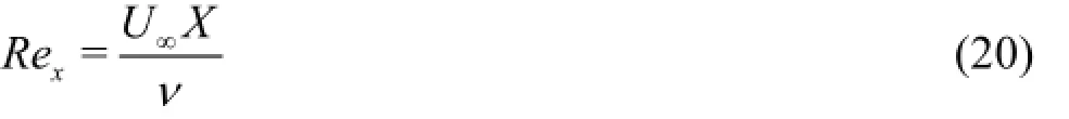
where the characteristic lengthX is the distance downstream from the start of the boundary layer， and the dimensionless wall distance is defined as

The velocity profiles at X =2.0 and 3.0 are chosen for comparison as in Fig.5（b） with different boundary layer Reynolds numbers. The results agree with the Blasius’s predictions［14］quite well， except deviations found in some places， caused by the limited size of the computational domain across the channel. As depicted in the figure， the larger the value of Rex， the further the upper boundary locatesand the more precise results are achieved. Besides，since at X =2.0， the boundary layer is thinner than that at X =3.0， comparatively better results are obtained.

2.2 Interior boundary simulation

In this part， the flows around a circular cylinder are simulated， and the diameterD of the cylinder is chosen as the characteristic length.

At a very low Reynolds number， the flow is steady and symmetrical. As the Reynolds number increases， the asymmetries and the time-dependence of the flow are developed， the famous Von Karman vortex street is formed， and fin［a15ll］y， the turbulence occurs. As pointed out by Qu et al.， when Re＞50， the unsteadiness arises spontaneously even though all the imposed conditions are being held steady and the vortex shedding appears behind the circular cylinder. Therefore， we simulate the flow at Re =40for the steady flow and at Re from 60 to 200 for the unsteady flows.

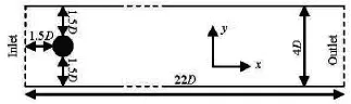
Fig.6 The geometric configuration and boundary conditions for the flow past a cylinder symmetrically placed in the channel

In the present study， a symmetrical computational domain with width of4D and length of22D is adopted， and the cylinder is located at （2D，2D）（as illustrated in Fig.6）. The boundary conditions are as follows: on the top and bottom sides， the symmetrical boundary conditions are applied， while on the cylinder surface， the no-slip boundary condition is imposed through the IB method. On the inlet （left side of the domain），u =1，v =0are given. At the far-field boundary， the pressure condition is applied.

In this flow， the pressure coefficient Cpis defined as

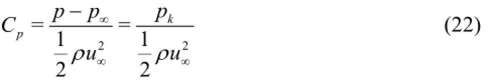
where p∞is the far-field pressure and pkis the pressure on the Lagrangian points. Then the dimensionless drag coefficient can also be defined as

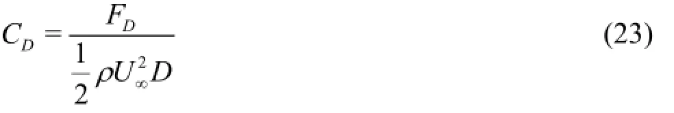
where FDis the drag force and can be easily calculated according to thex component of the force exerted on the Eulerian or Lagrangian points

It is interesting to note that both the contributions from the shear stress and the pressure distribution to the drag force could be obtained directly from the integral force［7］in the IB procedure.

Furthermore， for the unsteady flow， the shedding frequency could be represented as the Strouhal number，

where fwis the frequency in the lift force exerted on the cylinder.

In addition， we define L∞and L2as the norms of error as

whereN is the total number of the grid nodes andrepresents the solution at the finest grid density.

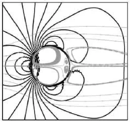
Fig.7（a） Pressure contour and streamlines for a stationary cylinder at Re =40by IBM

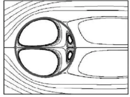
Fig.7（b） Streamlines for flow past a stationary cylinder at Re =40obtained by Wu et al.

2.2.1 Steady flow

Figure 7 shows the pressure contours and the streamlines of the flow and the corresponding results of Wu et al.［16］are also presented for comparison. It is obvious that the flow separates at the front stagnation point， and then merges down-stream， forming a pair of steady and symmetrical vortices. It is also interesting to note that the virtual flow also occurs inside the cylinder due to the fact that the whole domain is treated equally including that inside the cylinder.

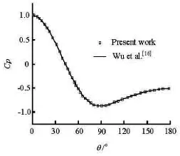
Fig.8 Pressure coefficient distribution on the cylinder surface at Re=40

The pressure coefficient Cpis plotted against the circumferential angle θfrom 0oto 180oin Fig.8. The results agree very well with the results of Wu et al.［16］. Then， another comparison is shown in Table 1 of the vortex length L/D ， which is the distance from the rear point of the cylinder to the stagnant point where the time-averaged streamwise velocity is zero. From the table， we can clearly see that the results are close to the previous data.

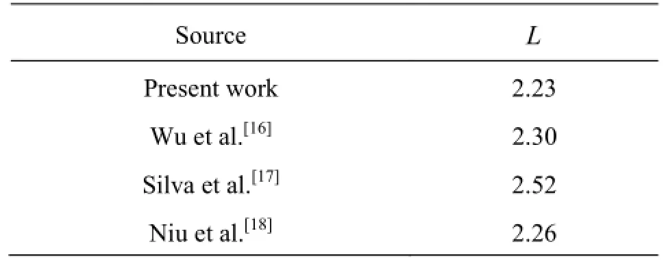
Table 1 Length of recirculation bubble at Re=40

For a balance between the grid resolution and the computational efficiency， the stretching grid approach is adopted in the following detailed analyses. As depicted in Fig.9， the finest constant grid spacing is imposed around the circle， while， a stretched grid is applied in the far region.

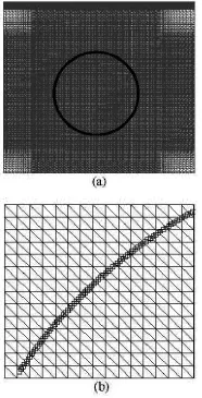
Fig.9 Illustration of stretched mesh， partial enlarged details see（b）

Then， the influences of the grid spacing on the convergence are analyzed for the case of Re =40.

We conduct a set of additional simulations with different grid sizes，h=0.04D，h=0.02D，h= 0.01Dand h=0.005D . In this part，h=0.005D is chosen as the baseline for comparison. The markerpoints are dense enough to avoid the influence of the marker points on the scheme accuracy. As depicted in Fig.10， a power between 1 and 2 is obtained for the norms （L∞and L2） of the streamwise and transverse velocity components predicted by the present method，which indicates that the approach has a spatial accuracy between first and second order. Considering the load and the accuracy of the calculation， hereinafter，h=0.01D is employed for further analyses.

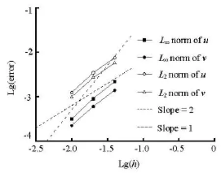
Fig.10L∞and L2norms of the error of the streanwise velocity and transverse velocity components versus the computational grid size

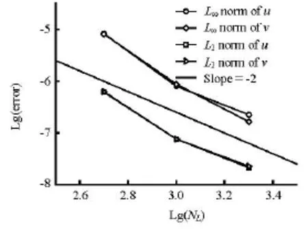
Fig.11L∞and L2norms of the error for the streamwise and transverse velocity components versus the number of IB points

On the other hand， the density of the Lagrangian points can influence the accuracy of the solution as well. To demonstrate it， we change the IB point number in this case and at the same time fix the other parameters. We make sure that the criterion of δs≤h/ 2［19］is always satisfied. The numbers of the IB points of 500， 1 000， 2 000 and 4 000 are selected， respectively. As shown in Fig.11， an error of O（N-2）is shown at certain stages based on the fixed grid spacing. However， this figure can change if the Cartesian grid resolution is changed.

2.2.2 Unsteady flow

Another interesting phenomenon is that the increase of the Reynolds number reduces the stability of the flow and the vortex shedding under certain values. The vorticity contours at Re =60，Re =100and Re=200are illustrated in Fig.12. In these figures，the Karman Vortex Street is fully developed and can be clearly observed. Meanwhile， associated with the results of steady flows， the criterion for vortex shedding in the flow around a cylinder should be40＜Re＜60， which agrees with the previous results［15］.

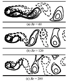
Fig.12 Instantaneous vorticity contours for cylinder. The solid lines denote positive vorticity， while the dash lines denote negative vorticity

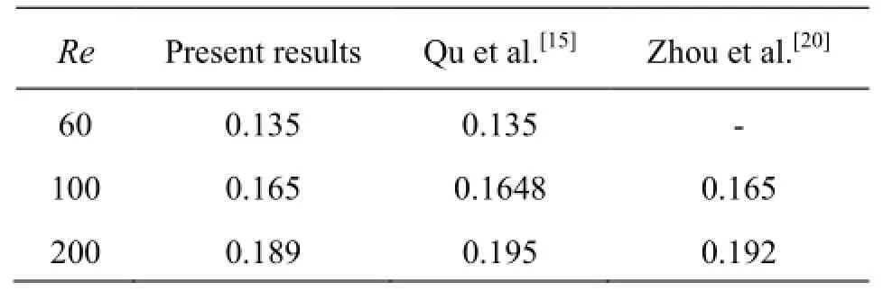
Table 2 The comparison of the numerical and experimental Strouhal numbers

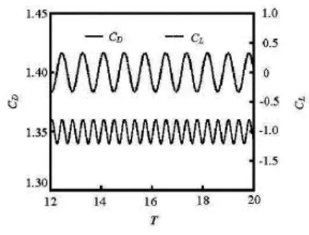
Fig.13 Lift and drag coefficients versus dimensionless time at Re=100

Table 2 shows theStnumbers at different Reynolds numbers， where we can obviously see that the results are consistent with published data. It shouldbe mentioned that Zhou［20］chose the turbulence model to simulate the 2-D flow， and his results indicate that its influence on the flows at a low Reynolds number could be neglected， otherwise， the 3-D turbulent structure should be considered. Figure 13 presents the dimensionless time （T=tU/L）evolution of the drag and lift coefficients atRe=100. The periodicity of the flow pattern is clearly revealed. It can be seen from the figure that the period of the drag coefficient is different from that of the lift coefficient and the period of the lift coefficient is about two times the period of the drag coefficient.

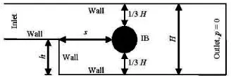
Fig.14 Geometry of flow around a cylinder behind backwardfacing step

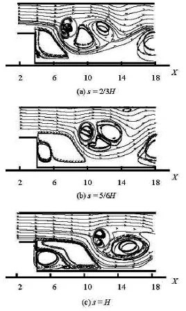
Fig.15 Streamlines in the vicinity of backward facing step with different locations of cylinder at Re=200

2.2.3 Flow around a cylinder behind backward facing step

For a practical application of the IB-CBS method，the flow around a cylinder behind a backward-facing step at Re =200with the channel expansion ER= H/h=2is selected for study （see Fig.14）. The cylinder surface is represented by 2 000 Lagrangian points in a uniform distribution. The computation starts with the given free stream velocity u=4um（y-h）·（H-y）/（H-h）2， whereyis the vertical coordinate of the inlet andumis the maximum velocity in the inlet.

The velocity vector fields are shown in Fig.15. Similar to the flow over a circular cylinder， a small recirculation zone is also seen behind the cylinder. The overall flow structure is in good agreement with the intuitive prediction. When the cylinder is inserted at different locations in the channel downstream of the backward facing step， wheres=2/3H，s=5/6H and S=Hare adopted， respectively， the different phenomena occur. And as depicted in Fig.15， an interesting phenomenon is that the larger the value ofs，the larger the corner eddies and the main recirculation region will be obtained. It should be mentioned that in the three cases， we just change the location of the cylinder with a fixed background grid. Therefore， in the circumstances where both the outer and inner geometries are complex， our method could be applied easily.

3. Conclusions

The novel direct forcing IB approach coupled with the CBS-FEM is proposed in this paper. The Eulerian （Cartesian） grid for the flow domain and the Lagrangian grid for the marker of the immersed boundary are applied following the methodologies of the immersed boundary method. In view of the FEM implementation and the coupling of the structure stress evaluation， the structured triangular grid is adopted. The background Cartesian grid is stretched for the balance between the accuracy and the efficiency.

A series of viscous incompressible flow simulations， including the Poiseuille flow， the laminar boundary layer flow， and the flow past a circular cylinder at different Reynolds numbers are performed in order to see the flexibility and the validity of the method. The obtained results agree well with the previous numerical and experimental data. Furthermore， the grid resolution tests indicate that with the method， a spatial accuracy between first and second order is achieved. We also show that the accuracy could be controlled by adjusting the number density of the mark points. A second power law could be achieved at certain stages. Finally， an interesting phenomenon is shown， that is. the location of the cylinder can influence the sizes and shapes of the corner eddy and the main recirculation region， by simulating the flow around a cylinder behind a backward-facing step. The method of this work can be applied further to fluid dynamics with complex geometries， moving boundaries， fluid-structure interactions， etc..

Acknowledgements

We gratefully acknowledge Peng Yan （Old Dominion University） and Lin Chao-An （National Tsing Hua University） for several insightful discussions on the direct forcing approach.

References

［1］ PESKIN C. S. Flow patterns around heart valves: A numerical method［J［. Journal of Computational Physics，1972， 10（2）: 252-271.

［2］ STERN F.， WANG Z. and YANG J. et al. Recent progress in CFD for naval architecture and ocean engineering［J］. Journal of Hydrodynamics， 2015， 27（1）: 1-23.

［3］ SHAO J. Y.， SHU C. and CHEW Y. T. Development of an immersed boundary-phase field-lattice Boltzmann method for Neumann boundary condition to study contact line dynamics［J］. Journal of Computational Physics， 2013， 234: 8-32.

［4］ PESKIN C. S. The immersed boundary method［J］. Acta Numerica， 2002， 11: 479-517.

［5］ MULEN R. The immersed boundary method for the（2D） incompressible Naiver-Stokes equations［D］. Master Thesis， Delft， The Netherlands: Delft University of Technology， 2006.

［6］ MITTAL R.， IACCARINO G. Immersed boundary methods［J］. Annual Review of Fluid Mechanics， 2005，37: 239-261.

［7］ LAI M. C.， PESKIN C. S. An immersed boundary method with formal second-order accuracy and reduced numerical viscosity［J］. Journal of Computational Physics， 2000， 160（2）: 705-719.

［8］ FADLUN E. A.， VERZICCO R. and ORLANDI P. et al. Combined immersed-boundary finite-difference methods for three-dimensional complex flow simulations［J］. Journal of Computational Physics， 2001， 161（1）: 30-60.

［9］ ZIENKIEWICZ O. C.， TAYLOR R. L. and NITHIARASU P. The finite element method， Vol. 3: Fluid dynamics［M］. 6th Edition， Oxford， UK: Butterworth-Heinemann， 2005.

［10］ NITHIARASU P. An efficient artificial compressibility（AC） scheme based on the characteristic based split（CBS） method for incompressible flows［J］. International Journal for Numerical Methods in Engineering，2003， 56（13）: 1815-1845.

［11］ ARPINO F.， MASSAROTTI N. and MAURO A. et al. Artificial compressibility based CBS solutions for double diffusive natural convection in cavities［J］. International Journal of Heat and Fluid Flow， 2013， 23（1）: 205-225.

［12］ NITHIARASU P. An arbitrary Eulerian Lagrangian（ALE） method for free surface flow calculations using the characteristic based split （CBS） scheme［J］. International Journal for Numerical Methods in Fluids，2005， 48（12）: 1415-1428.

［13］ SCHLICHTING H. Boundary layer theory［M］. Sixth Edition， New York， USA: McGraw-Hill， 1968.

［14］ STRAUSS D.， AZEVEDO J. L. F. On the development of an agglomeration multigrid solver for turbulent flows［J］. Journal of the Brazilian Society of Mechanical Sciences and Engineering， 2003， 25（4）: 315-324.

［15］ QU L.， NORBERG C. and DAVIDSON L. et al. Quantitative numerical analysis of flow past a circular cylinder at Reynolds number between 50 and 200［J］. Journal of Fluids and Structures， 2013， 39: 347-370.

［16］ WU J.， SHU C. and ZHANG Y. H. Simulation of incompressible viscous flows around moving objects by a variant of immersed boundary-lattice Boltzmann method［J］. International Journal for Numerical Methods in Fluids， 2010， 62（3）: 327-354.

［17］ SILVA L. E.， SILVEIRA-NETO A. and DAMASCENO J. J. R. Numerical simulation of two-dimensional flows over a circular cylinder using the immersed boundary method［J］. Journal of Computational Physics， 2003，189（2）: 351-370.

［18］ NIU X. D.， SHU C. and CHEW Y. T. et al. A momentum exchanged-based immersed boundary-lattice Boltzmann method for simulating incompressible viscous flows［J］. Physics Letters A， 2006， 354（3）: 173-182.

［19］ PENG Y.， LUO L. S. A comparative study of immersed-boundary and interpolated bounce-back methods in LBE［J］. Computational Fluid Dynamics， 2008， 8（1）: 156-167.

［20］ ZHOU Xing-gang， CHEN Xiao-peng and LIU Weiming et al. Two-dimensional simulation of flow around cylinder with multiple-relaxation-time lattice Boltzmann method［J］. Engineering Journal of Wuhan University，2012， 45（1）: 10-15（in Chinese）.

10.1016/S1001-6058（15）60528-5

E-mail: vonchaoyoung@mail.nwpu.edu.cn

（November 26， 2013， Revised May 10， 2014）

* Project supported by the National High Technology Research and Development Program of China （863 Program，Grant No. 2012AA011803）， the National Natural Scientific Foundation of China （Grant No. 11172241） and the University Foundation for Fundamental Research of NPU （Grant No. JCY-20130121）.

Biography: YANG Feng-chao （1989- ）， Male，Ph. D. Candidate

CHEN Xiao-peng，

E-mail:xchen76@nwpu.edu.cn