XIE Qiu-xia,ZHANG Long,WANG Xin-bing

(College of Mathematics and System Sciences,Xinjiang University,Urumqi Xinjiang 830046,China)

Abstract: In this paper,we extend the classical predator-prey model from a deterministic framework to a stochastic one and formulate it as a stochastic differential equation.Then,we obtain the global existence of a positive unique solution with positive initial value and the stochastically ultimate boundedness of the positive solution to the stochastic model is derived.

Key words:Stochastically ultimate bounded;White noise;It formula

0 Introduction

The dynamic relationship between predators and their preys has long been and will continue to be one of the dominant themes.Predator-prey is commonly modelled by using deterministic model.As the basic research of complex predator-prey models,prey dispersal models have already caused great interest by biomathematicians,and many significant work and monographies on species dynamics have been done[1−3].The most important subject of species diffusion models concentrate on the the extinction and the positive T-periodic solution[3],persistence and extinction[2].The classical model is sometimes used for modelling common phenomenon prey dispersal.Then the differential equations which describe the dispersal of the prey is:

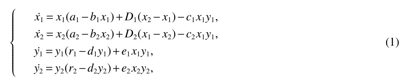
whereaiandridenotes the prey and predator intrinsic growth rate of patchi,respectively;eidenotes the conversion rate;bianddidenotes the density dependent coefficients of patchi;Direpresents the dispersal rate from patchjtoiand the dispersal occurs all of the time and happens simultaneously between two patches.

However,in all of above species dispersing systems,the variables in the model are completely determined by the parameters and its initial value,so we called this kind of model is a deterministic model[4].The deterministic model is established based on a thorough understanding of the behavior of the system,namely,to know the current state of the system can make a decisive response to future input.Deterministic models have two obviously shortcomings:on one hand,the general description of biological processes cannot reflect the biological especially the reality of observation data;on the other hand,it ignores the random perturbations occur in the stochastic environment with time going on.The most effective way to overcome these two shortcomings is to introduce stochastic fluctuating into the research deterministic model,i.e.the stochastic models.In fact,the species models are often subject to environmental noise;that is,parameters involved in species models are not absolute constants because of environmental fluctuations.In the 2000s,many authors introduce stochastic perturbation into deterministic models to reveal the effect of environment variability on the population dynamics in mathematical ecology[5−7].E.g.,Liu[7]studied a stochastic predator-prey model;discussed the permanent and the extinction of the solution in the stochastic environment.Liu[6]considered a nonlinear stochastic predator-prey system with Beddington-DeAngelis functional response,and showed the property of the positive equilibrium of the deterministic system under the stochastic environment.

As mentioned above,we can know that the stochastic model can provide more abundant information.All of us known that an accurate mathematical model is very useful to describe the predator-prey.So we establish the stochastic model,which is thinking about the biological background and the perturbations of stochastic environment,we establish the stochastic model.In this paper,we consider the perturbation on the parameter and this type of method is often called white noise.Known that a very few paper studied the stochastic perturbation on dispersal model.Motivated by these,we consider the stochastic perturbation on the prey dispersal rate of the parameters of the deterministic model.So the dispersal rateDi,riin model(1)replaced by

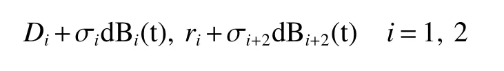
whereB1(t),B2(t),B3(t),B4(t)are mutually independent Brownian motions.σiand σi+2represents the intensities of the noise.Corresponding to the deterministic model system(1),the stochastic system takes the following from:

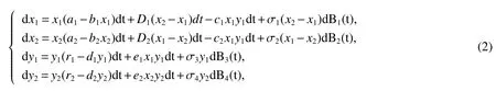
wherex1(t)andx2(t)stand for the prey population densities of patch 1 and 2 at time t respectively;y1(t)andy2(t)stand for the predator population densities of patch 1 and 2 at time t respectively;are positive parameters,i=1,2;j=1,2,3,4.

The rest of this paper is organized as follows.In Sec.1,we will give some preliminaries and assumption for system(2).In Sec.2,we state and prove the main results of this paper on the existence and uniqueness of positive solution and the boundedness in mean.

1 Preliminaries

Throughout this paper,unless otherwise specified,we letbe a complete probability space with a filtration{Ft}t≥0satisfying the usual conditions(i.e.it is right continuous andcontains all P-null set).LetB1(t),B2(t),B3(t),B4(t)denote the independent standard Brownian motions defined on this probability space.We denote byR4+the positive cone inR4,and also denote byx(t)=(x1(t),x2(t),y1(t),y2(t)),xi=xi(t),yi=yi(t)and

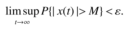
Definition 1[4]The SDE(2)is said to be stochastically ultimately bounded,if for any ε∈(0,1),there exist positive constants M such that for any initial valuethe solution of SDE(2)has the property that

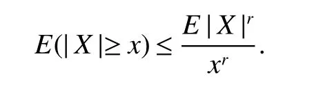
Lemma 1[4](Chebyshev inequality)For allr>0,x>0,we have

Assumption(H).bi>0,di>0i=1,2

2 Main results

Theorem 1Assume that assumption(H)holds,for any initial datax1(0)>0,x2(0)>0,y1(0)>0,y2(0)>0,there is a unique solution(x1(t),x2(t),y1(t),y2(t))to Eq.(2)ont≥0,and the solution will remain inwith probability one,namely,for allt≥0 almost surely.

ProofOur approach is inspired by the work of Luo[8]and Liu[9].Firstly,consider the equation

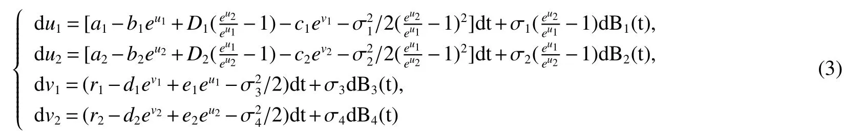
ont≥0,with initial valueu1(0)=lnx1(0),u2(0)=lnx2(0),v1(0)=lny1(0),v2(0)=lny2(0).It is easy to see that the coefficient of model(3)satisfy the local Lipschitz condition.Then there is a unique local solutionui(t),vi(t)on[0,τe)Therefore,by Itformulaxi(t)=eui(t),yi(t)=evi(t),i=1,2 is the unique positive local solution to(2)with initial valuexi(0)>0,yi(0)>0,i=1,2.

Now,we prove that τe= ∞ a.s.Letk0>0 be sufficiently large such that each component of(x1(t),x2(t),y1(t),y2(t))is no larger thank0.For each integerk≥k0,define the stopping time

where throughout this paper we set inf∅ = ∞.Obviously,τkis increasing ask→ ∞.Set τ∞=limk→∞τk,hence τ∞≤ τea.s.If we can show that τ∞= ∞ a.s.,then τe= ∞ a.s.In other words,to complete the proof all we need to show is that τ∞=∞ a.s.If this statement is false,then there is a pair of constantsT>0 and ε∈(0,1)such that

Hence there is an integerk1≥k0such that

Define a functionV:

here LV is a mapping fromdefined by

It follows from assumption(H).Hence,we have,

Therefore,we obtain

where β=max(max{|a1|,|a2|}+D1+D2,|r1|,|r2|).For anyt∈[0,T]andk≥k1,whence integrating both sides from 0 toT∧τk,and then taking expectations,yields

Using the well-known Gronwall inequality we get

Set Ωk={τk≤T}fork≥k0,and by(6),we have,P(Ωk)≥ ε.Note that,for every ω ∈ Ωk,there is some i such thatxi(τk,Ωk)or yi(τk,Ωk)equals k.Hence we have

Lettingk→∞leads to the contradiction

So we must therefore have τ∞=∞ a.s.,whence the proof is complete.

Theorem 1 shows that the solution of system(2)will remain in the positive conewith probability one.As we all know,because of the limit of the resource the ultimate boundedness of the solution x(t)is more desire,which can be guaranteed by the following two results.

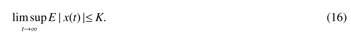
Theorem 2Assume that assumption(H)holds,for any given initial valuex(0)∈there exists a positive numberK>0 such that the solution x(t)of SDE(2)has the following property:

ProofBy theorem 1,the unique solutionx(t)of system(2)will remain infor allt∈R+with probability one.Defineas in(7).By Itformula,we have

where LV is a mapping fromas in(9).

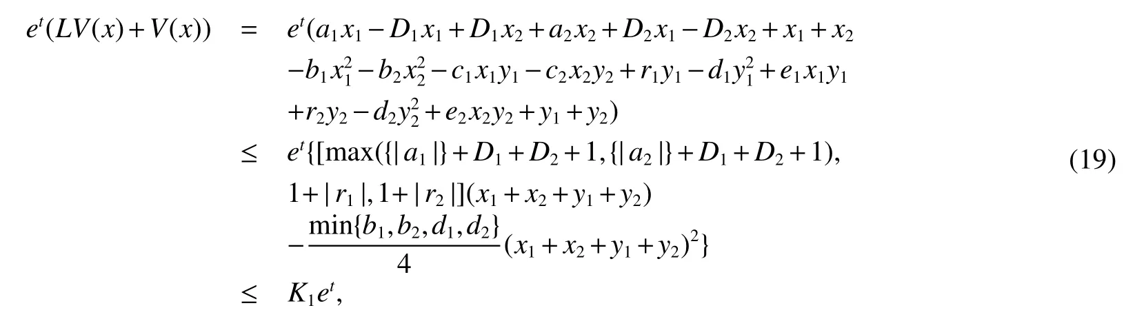
w h e r et h e r e f o r e,w e h a v e

For each integerk≥|x(0)|,define stopping time

Integrating both side of the inequality(20)from 0 tot∧τk,and then taking expectations,yields

Lettingk→∞,clearly τ∞→∞ yields

This implies

Note that

So

Thus

This implies

and the assertion(16)follows by settingK=2K1.

Theorem 3Assume that assumption(H)holds,solutions of SDE(2)are stochastically ultimately bounded.

ProofBy theorem 2,we have(16)is satisfied.Now,for any ε>0,LetThen by Chebyshev’s inequality,

Hence

This implies

as required.

Remark 1We should like to point out that the permanence of a deterministic model implies that population of species in the system is bounded above zero and below certain number while the concept of stochastically permanent implies that the sum of species population in the stochastic system is bounded above zero below certain number with probability arbitrary close to 1.