HaiBo Wang, MingGuo Ma

1. Heihe Remote Sensing Experimental Research Station, Cold and Arid Regions Environmental and Engineering Research Institute, Chinese Academy of Sciences, Lanzhou, Gansu 730000, China

2. Key Laboratory of Remote Sensing of Gansu Province, Cold and Arid Regions Environmental and Engineering Research Institute, Chinese Academy of Sciences, Lanzhou, Gansu 730000, China

3. School of Geographical Sciences, Southwest University (Beibei District), Chongqing 400715, China

Comparing the seasonal variation of parameter estimation of ecosystem carbon exchange between alpine meadow and cropland in Heihe River Basin, northwestern China

HaiBo Wang1,2*, MingGuo Ma3

1. Heihe Remote Sensing Experimental Research Station, Cold and Arid Regions Environmental and Engineering Research Institute, Chinese Academy of Sciences, Lanzhou, Gansu 730000, China

2. Key Laboratory of Remote Sensing of Gansu Province, Cold and Arid Regions Environmental and Engineering Research Institute, Chinese Academy of Sciences, Lanzhou, Gansu 730000, China

3. School of Geographical Sciences, Southwest University (Beibei District), Chongqing 400715, China

Grasslands and agro-ecosystems occupy one-third of the global terrestrial area. However, great uncertainty still exists about their contributions to the global carbon cycle. This study used various combinations of a simple ecosystem respiration model and a photosynthesis model to simulate the influence of different climate factors, specifically radiation, temperature, and moisture, on the ecosystem carbon exchange at two dissimilar study sites. Using a typical alpine meadow site in a cold region and a typical cropland site in an arid region as cases, we investigated the response characteristics of productivity of grasslands and croplands to different environmental factors, and analyzed the seasonal change patterns of different model parameters. Parameter estimations and uncertainty analyses were performed based on a Bayesian approach. Our results indicated that: (1) the net ecosystem exchange (NEE) of alpine meadow and seeded maize during the growing season presented obvious diurnal and seasonal variation patterns. On the whole, the alpine meadow and seeded maize ecosystems were both apparent sinks for atmospheric CO2; (2) in the daytime, the mean NEE of the two ecosystems had the largest values in July and the lowest values in October. However, overall carbon uptake in the cropland was greater than in the alpine meadow from June to September; (3) at the alpine meadow site, temperature was the main limiting factor influencing the ecosystem carbon exchange variations during the growing season, while the sensitivity to water limitation was relatively small since there is abundant of rainfall in this region; (4) at the cropland site, both temperature and moisture were the most important limiting factors for the variations of ecosystem carbon exchanges during the growing season; and (5) some parameters had an obvious characteristic of seasonal patterns, while others had only small seasonal variations.

ecosystem carbon flux; ecosystem respiration; gross ecosystem productivity; climatic factors; alpine meadow; farmland ecosystem

1　Introduction

Grasslands and agro-ecosystems occupy one-third of the global terrestrial area, and play a significant role in the uptake of atmospheric CO2and its transformation to biomass and soil organic matter (Follett and Schuman, 2005). Alpine meadows are widely distributed on the Qinghai-Tibetan Plateau (QTP), with an area of about 1.2×106km2, which amounts to 30.92% of the total rangeland of the Tibet Autonomous Region in China (Xu et al., 2005). Arid regions occupy another one-third of the area of China. The plants in the arid regions are very sensitive to soil moisture, since the precipitation is limited in those areas. Plant photosynthesis will decline under dry conditions, and this is related to the variation of stomatal conductance with water stress (Anthoni et al., 2002).

Quantifying the contribution of various ecosystems to the regional and global carbon cycles is a fundamental task for the carbon cycle science (Lieth, 1975). However, less agreement exists with respect to the contributions of grassland and cropland ecosystems to these cycles (Gilmanov et al., 2010). Grasslands are typically characterized as weak sinks, or as approaching a carbon-neutral state, whereas croplands are considered moderate to strong sources of atmospheric carbon based on indirect measurements of biomass and soil organic matter inventories (Smith and Falloon, 2005). However, Gilmanov et al. (2010) argued that 80% of the non-forest sites were apparent sinks for atmospheric CO2, and although agricultural fields may be predominantly sinks for atmospheric CO2, they do not necessarily increase their carbon stock because of the harvest and off-site transport of the crops.

Worldwide concern with global climate change and its effects on our future environment requires a better understanding and quantification of the processes contributing to those changes (Fang et al., 2001). The response of vegetation to the environment is a key global climate change issue that scientists are investigating by means of measurements and models on short- and long-term scales (Law et al., 2002; Gilmanov et al., 2010). Previous studies about the response of terrestrial ecosystems to environment conditions mainly focused on the measurements of aboveground production in relation to temperature, precipitation, and empirical estimates of evapotranspiration (Law et al., 2002). The eddy-covariance (EC) technique (Wofsy et al., 1993) has become the main method for sampling ecosystem carbon, water, and energy fluxes at hourly to inter-annual time scales (Baldocchi et al., 2001). Bai et al. (2012) analyzed the impact of solar radiation on net ecosystem exchange (NEE) in grassland and cropland ecosystems with different canopy structures and climate conditions, and indicated that NEEs were more negative (more carbon uptake) in grasslands and maize croplands under cloudy skies compared to clear skies. Besides radiation and temperature, which are taken into account in the light-temperature response function, water is also a very important factor that influences ecosystems' productivity (Boyer, 1982). However, since the light-response function does not include the factor of moisture, many previous studies did not account for the effect of water in the estimation of ecosystems' productivity.

The EC NEE flux partitioning algorithm is used to estimate ecosystem respiration (ER) and gross ecosystem carbon uptake (GEP) from the NEE according to the defining equation NEE = ER - GEP (Reichstein et al., 2005). A commonly used technique is estimation of the parameters of NEE with climatic variables, such as temperature, light, and moisture (Reichstein et al., 2005). The quantum yield (α) and maximum photosynthetic capacity (Pmax) are important parameters of the light-response function for describing ecosystem photosynthetic activity, and they have received worldwide attention in the evaluation of the global carbon budget (Ruimy et al., 1995). The seasonal and inter-annual variations of ecosystem α and Pmaxand their responses to temperature have been studied for a range of ecosystems (Wofsy et al., 1993; Hollinger et al., 1999). However, most studies have focused on forest ecosystems (Wofsy et al., 1993; Hollinger et al., 1999; Zhang et al., 2006), and such studies are still insufficient on non-forest ecosystems, especially cropland ecosystems. Some example cases are as follows: Xu et al. (2005) and Zhang et al. (2007) analyzed the relationship between NEE and photosynthetically active radiation (PAR) of the alpine meadow ecosystem in the QTP using continuous carbon flux data, and found that the apparent α and Pmaxexhibit large variability. Gilmanov et al. (2010) also found that there is a wide range of variability for the light-response parameters of non-forest terrestrial ecosystems (grasslands and agro-ecosystems), and the maximum values of GEP in nonforest terrestrial ecosystems can even surpass the productivity of forests under optimal conditions (Gilmanov et al., 2010). However, these works did not consider the uncertainty in the estimation of parameters.

Because model parameters do vary by plants and species as a result of genetic or environmental variation, the underlying mechanisms between the photosynthesis process and environment response have not yet been clarified fully, and thus large uncertainties are present in both the data and the models. To improve the capability of ecosystem models to analyze environment responses, these uncertainties need to be quantified and reduced. The Bayesian approach can then be employed to update the parameter dis-tributions when new information becomes available (Van Oijen et al., 2005). The Bayesian approach can produce reliable estimates of parameter and predictive uncertainty. It can also provide the modeler with valuable qualitative information on the shape of the parameter and predictive probability distributions (Gallagher et al., 2007).

Our studies analyzed the effect of different environmental factors (radiation, temperature, and soil moisture) on the ecosystem carbon exchange estimation, and the dynamic variation patterns of the parameters during the growing season of alpine meadow and cropland ecosystems in an inland river basin of China using flux tower measurements taken in 2009. The ecosystem carbon flux model was calibrated using a Bayesian approach in order to identify the seasonal variations of parameters and their uncertainty. Our research could thus produce measurement-based estimates of the role of non-forest ecosystems as net sinks or sources for atmospheric CO2, and may provide a basis for carbon balance evaluation and parameters selection for the carbon flux model. Analyzing the carbon budget and the control factor in these sites is important to understand present and future climate change, vegetation dynamics, and global warming.

2　Methods and materials

2.1Sites and data

Our study sites, the A'rou (AR) freeze/thaw observation station (100°28′E, 38°03′N; 3,032.8 m a.s.l.) and the Yingke (YK) oasis station (100°25′E, 38°51′N; 1,519 m a.s.l.), are located in the Heihe River Basin, the second largest inland river basin in the arid region of northwestern China (Li et al., 2009). The AR station is located on the upper stream of the Heihe River, which is located in the southeastern area of the QTP; the main vegetation type in the AR station is alpine meadow. The YK site is located in the central area of the Yingke irrigation oases along the middle stream of the Heihe River, and the primary crop at the YK station was seeded maize. The mean annual temperatures at AR and YK are 0.7 °C and 6.5 °C, and their average annual precipitations are 400 and 125 mm, respectively. The observation variables in these sites can be found in Li et al. (2009).

We obtained time series of temperature, solar radiation, and soil moisture in 2009 at the AR and YK stations. We also analyzed the EC data measured at the two stations in 2009. Components of the wind vectors and temperature were measured using a three-dimensional sonic anemometer (CSAT3, Campbell Scientific, Inc., Logan, UT). Water vapor density and CO2mixing ratios were measured using an open-path infrared gas analyzer (Li-7500, LiCor Inc., Lincoln, NE). The sampling frequency was 10 Hz. The energy balance ratio was approximately 87% at AR station and 86% at YK station. The raw 10 Hz EC data were processed to obtain half-hourly flux data using the flux post-processing software EdiRe (University of Edinburgh, UK). The flux data processing steps included despiking, coordinate rotation, time-lag correction, frequency-response correction, and WPL correction (Zhang et al., 2010). The detailed data quality control processes can be found in Zhang et al. (2010).

2.2Model descriptions

Based on the EC observed carbon flux data and climatic variables, the NEE is an observation that represents the sum of GEP and ER. In this study, we employed a commonly used temperature-dependent exponential model, Van't Hoff's ecosystem respiration equation (Van't Hoff, 1898) to simulate the ER:

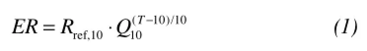
where ER is the ecosystem respiration, µmol/(m2·s); Rref,10is the basal respiration rate at 10 °C, µmol/(m2·s); Q10(dimensionless) is the change in the rate of respiration with temperature; and T is the air temperature, °C.

To analyze the sensitivity of ecosystem production to certain environmental factors (i.e., radiation, temperature, and soil moisture), four combinations of factors based on the Michaelis-Menten equation were evaluated: (1) only considering the radiation limitation on photosynthesis (Equation 2); (2) containing both radiation and temperature (Equations 2 and 3); (3) containing both radiation and soil moisture (Equations 2 and 4); and (4) containing radiation, temperature, and soil moisture (Equations 2, 3 and 4).

where PAR is the incident photosynthetic photon flux density, µmol photon/(m2·s); α is the ecosystem apparent quantum yield, µmol CO2/(μmol PAR); and Pmaxthe ecosystem maximum photosynthetic capacity, µmol CO2/(m2·s). The Michaelis-Menten equation only considered the radiation limitation on photosynthesis. Since temperature and soil moisture are also known to limit photosynthesis, which can simply be included by modifying the α by the fractional multiplier f(T) or (and) f(W) in the prior Michaelis-Menten equation, the f(T) and f(W) represent the limitation of temperature and soil moisture, respectively, on photosynthesis.

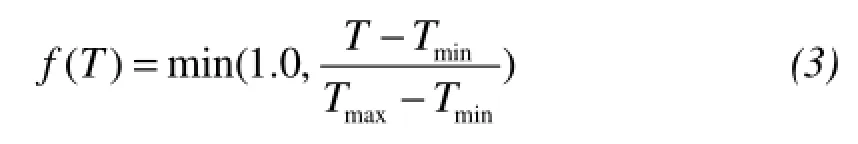
where the parameters of Tmaxand Tminin f(T) represent a fractional reduction for α as a linear function of temperature T. Similarly, the Wmaxand Wminin f(W) reflect the limitation of water.

2.3Ecosystem photosynthetic parameters estimation and uncertainty analysis

The Bayesian approach was used in estimating the parameters of the photosynthetic models. The technique has already been widely used in ecosystems models (e.g., Braswell et al., 2005; Van Oijen et al., 2005). According to Bayesian theory, posterior probability density functions (PDFs) of model parameters θ given the existing data, denoted as P(θ |Data), can be obtained from prior knowledge of the parameters and information generated by comparison of simulated and observed variables, and can be described by Equation (5) (Mosegaard and Sambridge, 2002):

where P(Data) is the probability of observed data, and P(Data|θ) is the conditional probability density of observed data with prior knowledge, also called the likelihood function for parameter θ.

Given a collection of N measurements, the likelihood function (L) can be expressed by Equation (6):

where σ represents the SD of the data-model error, Xirepresents the ith of N measurements, and ηiis the model-derived estimate of a measurement.

The posterior PDFs for the model parameters were generated from prior PDFs P(θ) with observation data by a Markov Chain Monte Carlo (MCMC) sampling technique. Herein, the Metropolis-Hasting algorithm (Metropolis et al., 1953; Hasting, 1970) was adopted to generate a representative sample of parameter vectors from the posterior distribution. We ran the MCMC chains with 50,000 iterations each, and regarded the first 15,000 times as the burn-in period for each MCMC run. All accepted samples from the runs after burn-in periods were used to compute the posterior parameter statistics of the models.

2.4Experiment configuration

Combining the ecosystem respiration equation with the photosynthetic productivity model limited by different environmental factors produced four ecosystem carbon exchange models. Table 1 shows the four combinations of ecosystem carbon exchange models and their limiting factors.

To find the model that best explains the carbon flux observations, the MCMC method was used to estimate parameters for all combinations of the models, for priors, assuming those parameters were in uniform distribution; we set the likely range of these values based on literature estimates. We also used the Bayesian information criteria metric (BIC), log likelihood (Ln(L) or LL), and the correlation coefficient (R2) to help select the best set of models among the four models and determine which one was most consistent with the observations, while using the minimal number of parameters. BIC, also known as the Schwarz criterion (Schwarz, 1978), can be used to calculate the information loss in each step within conditional Bayesian inversion (Zobitz et al., 2011). A lower BIC is considered to have less information loss with better model performance (Braswell et al., 2005).

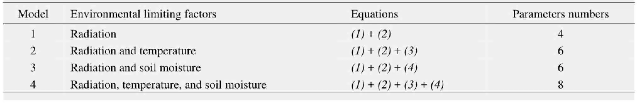
Table 1 The environmental limiting factors and formulas and parameters for different models

3　Results

3.1Seasonal variation of environmental conditions Figure 1 shows the changes of mean air temperature, integrated precipitation, and global solar radiation at the AR and YK sites in every month during the study period. Different seasonal variations of environmental factors in the alpine meadow and oasis cropland ecosystems are shown in the figure. In the alpine meadow of the AR site, the temperature was low and the precipitation was abundant during the growing season, whereas the opposite was true in the YK oasis cropland ecosystem: the temperature washigh and there was little rainfall. In 2009 the annual average temperatures were -0.3 °C and 7.8 °C at the AR site and YK site, respectively, and the yearly integrated rainfall was 450.5 mm and 68.7 mm. Thus, the water supply for maize in the YK site mainly depended on irrigation, while the AR grassland depended on precipitation. The seasonal variations of radiation were small in the two sites.

3.2Diurnal and seasonal variation patterns of NEE Figure 2 reveals the averaged diurnal variation of NEE during the growing season (from June to October) and the whole year of 2009 (NEE toward atmosphere is positive, denoting carbon release; NEE toward vegetation is negative, denoting carbon uptake). From this figure, we can see that the NEE of alpine meadow and seeded maize during the growing season presented obvious diurnal variation patterns. During nighttime, the whole ecosystem was a carbon source because of ecosystem respiration, while during the daytime, as the plants photosynthesized, the whole ecosystem turned into a carbon sink around at 08:00 (local time), and reached its diurnal maximum carbon assimilation usually at 13:00-14:00 (local time). On the whole, the alpine meadow and seeded maize ecosystems were both apparent sinks for atmospheric CO2, which accords with the viewpoint of Gilmanov et al. (2010).

The diurnal maximum carbon assimilation of the alpine meadow and seeded maize ecosystems varied with the growing stages. It was highest in July, when the vegetation was in peak growth [-13.32 μmol CO2/(m2·s) for grassland, and -39.47 μmol CO2/(m2·s) for cropland], and was lowest in October, which was the withering (or harvesting) period [-1.68 μmol CO2/(m2·s) for grassland, and -1.64 μmol CO2/(m2·s) for cropland].

Figure 1 Seasonal variations of temperature, precipitation, and radiation at the YK and AR sites

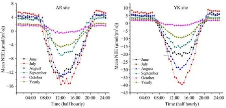
Figure 2 Diurnal and seasonal variation patterns of NEE at the AR and YK sites

3.3 Sensitivity of simulated carbon fluxes to temperature and moisture

We used the data from the AR and YK sites in the whole year of 2009, and simulated the ecosystem carbon exchange with the four models described in Table 1. We used the Bayesian approach to calibrate these parameters, and the simulated results are shown in Table 2.

The results revealed that all four combinations of the equations were generally able to adequately capture most of the observed variability of the data. The patterns of variation in the carbon flux estimates in the alpine meadow and arid cropland ecosystems mainly depended on radiation, precipitation, and temperature; however, there were some differences in the main limiting factors in these two ecosystems. For both the AR and YK sites, when we only contained the effect of radiation on NEE simulation (Model 1), the R2was relatively low, the log likelihood (LL) was small, and the BIC was high, which indicated a relatively poor performance of the model. When accounting for the soil moisture limitation on NEE (Model 3), the performance was very close to the radiation limitation on NEE (Model 1) - only a slight improvement compared with Model 1. However, there was some difference between the AR and YK sites when the temperature factor was included (Models 2 and 4). For the AR site, Models 2 and 4 had the lowest BICs, suggesting a high temperature limitation and a relatively low water limitation on NEE at the AR site. In contrast, for the YK site, Model 4 had the best performance and the BIC of Model 2 was larger than that of Model 4, which suggested a high water and temperature limitation on NEE at the YK site.

From these results, we can conclude that for the alpine meadow ecosystem in AR, the temperature was the main limiting environment factor for the NEE estimation, whereas the sensitivity of NEE to soil moisture was low. However, for the cropland ecosystem in YK, soil moisture and temperature were important limitations on NEE. This phenomenon can be attributed to the abundant precipitation at the AR station during the study period, making the soil moisture very high during the growing season (Figure 3). Thus, the photosynthesis of the grassland was not sensitive to water stress. However, the precipitation was insufficient at the YK station, which is why irrigation is the main source for agricultural water in that area. The NEE in the maize cropland was very sensitive to these irrigation events.

秀容月明成亲那天，天蓝蓝的，门前的桃花开得正艳。娶亲的队伍吹吹打打，从东大街到西大街，又从西大街回到东大街。

Table 3 illustrates the "most likely" parameter values estimated by the MCMC method for the different models. Some of photosynthesis parameters had large variations when estimated by the different models, but others had only slight variations. For the grassland at the AR site, the differences in the photosynthesis parameters between the values estimated by Models 1 and 3, and Models 2 and 4 were small; however, when we compared Model 1 with Models 3, 2, and 4, the variation was large. This indicated that the ecosystem productivity at the AR site was not sensitive to the soil moisture but was sensitive to the temperature. When we compared the photosynthesis parameters between the two plant species, the variations of the Pmaxand α between them were large; overall, the photosynthetic capacity of the C4 cropland was larger than that of the C3 grassland.

3.4Uncertainty analysis of model parameters

Assuming the model parameters had uniform distributions, we obtained the posterior distributions of the model parameters through the Bayesian approach. To summarize the uncertainty of the parameters from the posterior distributions of each parameter, we produced PDF graphs to visually explore the parameter uncertainties. Additionally, we calculated the mean vectors and the variations for each of the parameters for the "optimal" model of each site.

Figure 4 shows PDF graphs of the "optimal" model fitted with observations for the AR and YK sites. Differences in the shapes of the posterior distributions of the parameter vectors indicate a difference in the most likely parameter for which the model fits the observations. Figure 5 shows plots of the posterior parameter distributions corresponding to the means and 95% CIs after calibration with NEE data from the AR and YK sites. This figure makes it possible to visualize differences in the parameter PDFs, since the intervals of the parameters reveal the dispersion and symmetry of the parameter distributions. The main photosynthetic parameters (e.g., Rref,10, Q10, α, Tmin, Wmax, and Wmin; Figure 4) were updated well by the MCMC procedure, as demonstrated by narrow CIs and low variability for these parameters (Figure 5). Also, from Figure 4, the posterior means of the parameters were different from the means specified by their prior distributions (uniform distribution, x-coordinate of Figure 4), indicating that these parameters were more identifiable with less informative priors, and were well constrained by the observation data.

However, it was not the same for other parameters, such as Pmaxand Tmax. In contrast, the posterior distributions of these parameters had relatively broad CIs (Figure 5), and thus had greater uncertainty than the other parameters. Additionally, there were some differences between the AR and YK sites in the variability of some parameters. For example, the variability of Pmaxat the YK site was larger than that of the AR site, while the variability of Tminat the AR site was larger than that of the YK site. This was probably due to differences in site characteristics such as vegetation types, rainfall, air temperature, etc..

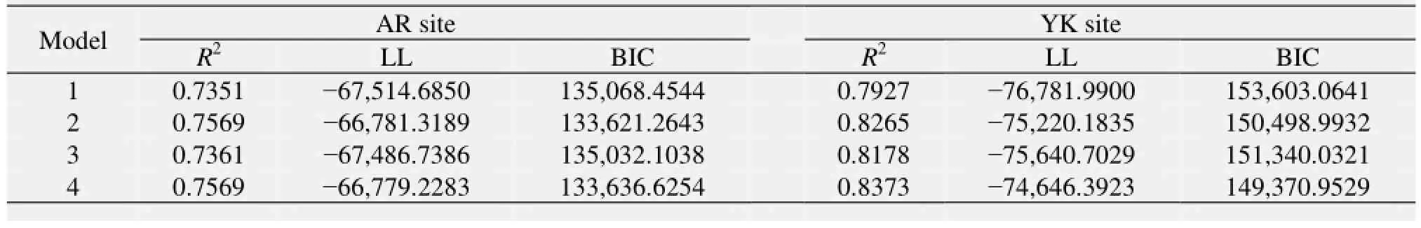
Table 2 Accuracy evaluation of the annual simulation by four carbon flux models

Figure 3 Seasonal variation of simulated half-hourly precipitation and 10-cm soil moisture

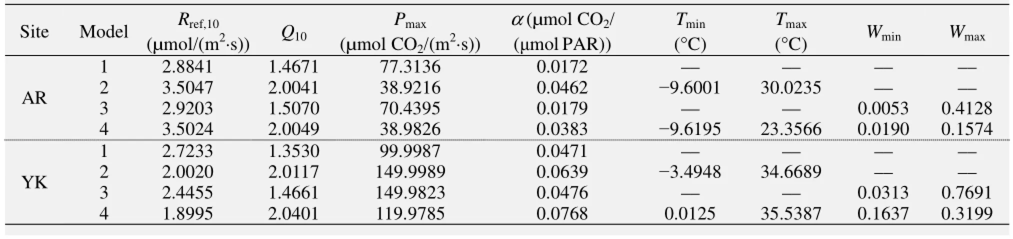
Table 3 The best parameter values estimated by different models at the AR and YK sites

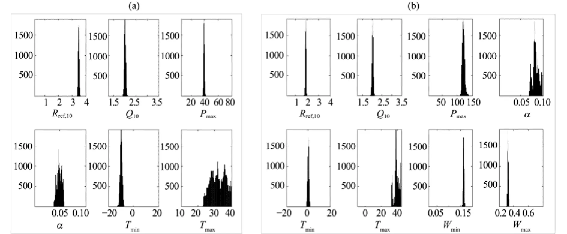
Figure 4 PDFs graphs of parameter vectors of Model 2 for the AR site (a) and those of Model 4 for the YK site (b)

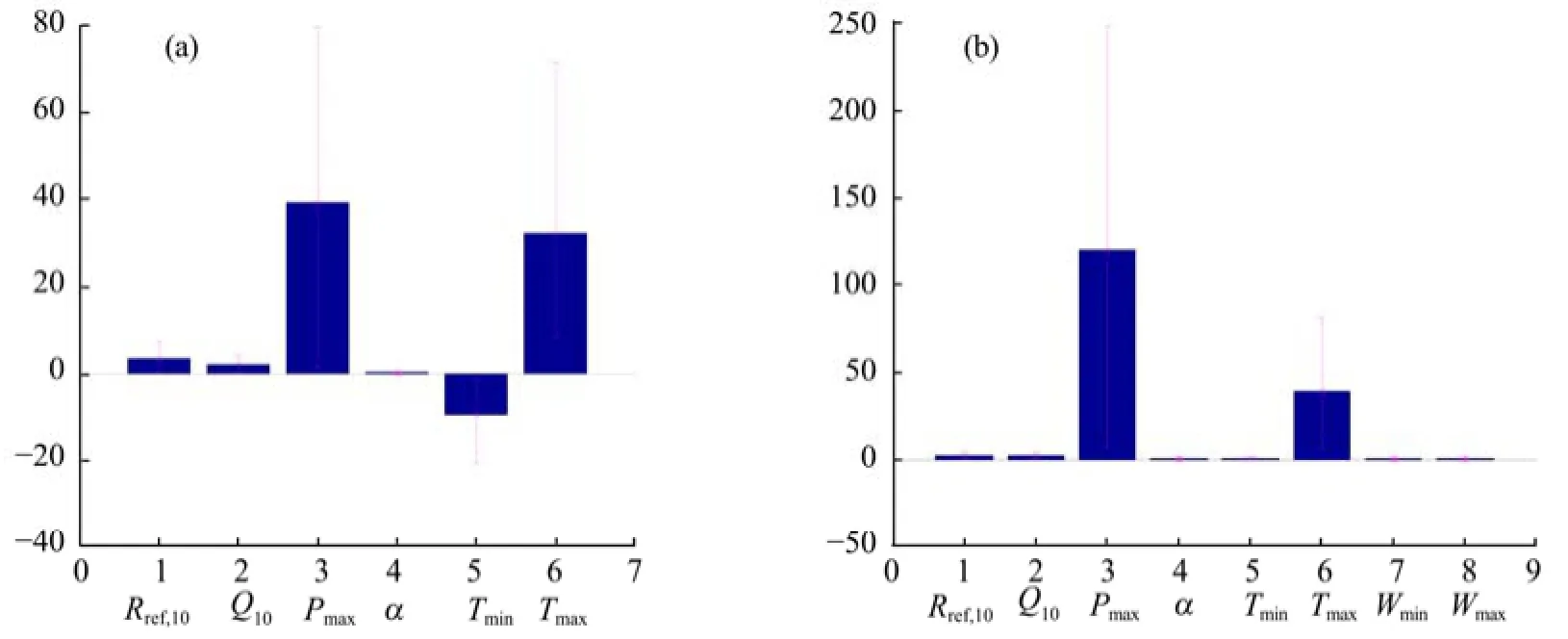
Figure 5 Posterior means and 95% confidence intervals (CIs, i.e., 2.5th and 97.5th percentiles) estimates of parameter vectors for Model 2 at the AR site (a) and those of Model 4 at the YK site (b)

3.5Variations in simulated ecosystem carbon flux

The NEE of grassland and farmland ecosystems during the growing season (from June to October) at the AR and YK sites was simulated with the above four models, and the MCMC approach was applied to estimate the photosynthesis parameters. The simulated results by different models are shown in Table S1 (see the supporting information). Comparing these seasonal variation results with the annual results in Table 2, the accuracy of the seasonal variation simulation during the growing season period (in July and August) was better than the annual results, and decreased as the plants matured and withered. Similar to the annual results, the temperature-limited Models 2 and 4 yielded the best results, and few improvements were found in the water-limited Models 1 and 3 at the AR site, indicating that the grassland was not sensitive to the soil moisture during the growing season. However, at the YK site, the model performance improved when the water limitation factor was considered, which indicated that the ecosystem carbon fluxes were sensitive to both temperature and soil moisture. Table S1 also reveals that the accuracy of the simulation declined as the plants grew. It was highest during the peak growth period (in July), and declined with the maturing and withering of the plants.

Figures 6 and 7 show the simulated daily NEE during the growing season by Model 4 with the optimal model parameter vector. The model could generally well simulate the seasonal patterns of the ecosystem carbon exchanges. However, as the plants grew, the accuracy of the NEE simulation decreased, and in some cases the results showed large uncertainty in simulating the peaks of photosynthesis.

Figures S1 and S2 in the supporting information illustrate the seasonal dynamic patterns of the optimal parameters estimated by the MCMC method during the grassland and cropland growing seasons. We found that some of the parameters had obvious seasonal dynamic variation, such as Rref,10, Q10, Pmax, α, Tmin, and Tmax, which increased during the initial growth of the plants and decreased as the plants matured and withered. For example, the Pmaxwas the highest in July, when the vegetation was in peak growth, and it was low in October, as the vegetation was withering.

There were also some variations among the different models within the same months, such as the parameters were different when contained the temperature-limited factor or not in estimating the NEE. However, these variations in the same months were relatively small compared with the seasonal variations.

4　Discussion

4.1Photosynthetic parameters comparison

Xu et al. (2005) used a method similar to our Model 1 to estimate the values of α and Pmaxat various stages of alpine meadow growth at Damxung, another alpine meadow ecosystem on the QTP. Table 3 presents a comparison between our Model 1 results and Xu et al.'s results. The α and Pmaxvalues at the AR site were larger than those at Damxung. The largest values of α and Pmaxat Damxung were, on average, 0.0244 µmol CO2/(μmol PAR) and 10.0909 µmol CO2/(m2·s), respectively, during the peak growth period when all the environmental factors were optimal. However, the α and Pmaxin our study were 0.06506 µmol CO2/(μmol PAR) and 31.659 µmol CO2/(m2·s), respectively. Also, the maximum α in AR occurred in July, while the maximum of α in Damxung occurred in August. This is because of the elevation of AR (3,033 m a.s.l.) is lower than Damxung (4,333 m a.s.l.), and the phenology of AR is earlier than that of Damxung.

Figure 6 Observed vs. simulated daily NEE during the growing season by Model 4 at the AR site. (a) in June; (b) in July; (c) in August; (d) in September

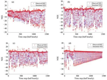
Figure 7 Observed vs. simulated daily NEE during the growing season by Model 4 at the YK site. (a) in June; (b) in July; (c) in August; (d) in September

Zhang et al. (2007) conducted similar research at the Haibei station (101°19′E, 37°37′N; 3,200 m a.s.l.) on the QTP, where the environmental conditions and location are very similar to the AR site. Some similar results were reported at these two alpine sites. Those researchers analyzed three vegetation types (alpine Kobresia humilis (C. A. Mey) Serg. meadow, alpine Potentilla fruticosa shrubland, and alpine Kobresia tibetica Maxim. wetland) in the growing season (from June to September). They found that the maximum α at the K. humilis meadow [0.09409 µmol CO2/(μmol PAR)] and the P. fruticosa shrubland [0.08091 µmol CO2/(μmol PAR)] was higher than that of the alpine meadow at AR site, while the maximum α at the alpine K. tibetica wetland [0.05705 µmol CO2/(μmol PAR)] was close to that of the AR site. The maximum α and Pmaxat the K. humilis meadow also occurred in August, and those of the other two vegetation types in July, which was similar to the AR site. The maximum Pmaxat the K. humilis meadow was 25.95091 µmol CO2/(m2·s), which was close to our result at the AR site.

For comparison with other grassland ecosystems in the world, Andrew et al. (2001) used the EC data in a tall grass prairie site in north-central Oklahoma, USA, where the estimated α was 0.0348 µmol CO2/(μmol PAR) when there was no moisture stress during the peak growth; when moisture stress conditions prevailed, α was considerably smaller [on average 0.0234 µmol CO2/(μmol PAR)]; when plants were in the senescence period, α was only 0.0114 µmol CO2/(μmol PAR). These values agreed with the value estimated by Model 1 in this study.

For comparison with other cropland ecosystems in the world, such as the maize crop at Bondville, USA (Gilmanov et al., 2010), the α and Pmaxwere 0.03182 µmol CO2/(μmol PAR) and 72.7273 µmol CO2/(m2·s), respectively, which were close to the seeded maize at the YK site in our study. However, the Pmaxof seeded maize in our results was higher than that of soybeans [12.5955 µmol CO2/(m2·s)] at Rosemount, USA and sown pasture [18.2909 µmol CO2/(m2·s)] at Lacombe, Alberta, Canada (Gilmanov et al., 2010). Since the crop type at the YK site was seeded maize, the canopy height of which was more than 2.0 m and the maximum leaf area index (LAI) was about 4.0–5.2 m, the photosynthesis capability was larger than that of an ordinary maize crop.

4.2Seasonal patterns of parameter dynamics

The photosynthetic parameters can represent physiological characteristics of ecosystems which change through time with phenology and environmental conditions such as radiation, temperature, and moisture. Thus, in our study these parameters exhibited seasonal variations during the year (Figures S1 and S2). The seasonal dynamics of these parameters were related to the variation of the environmental conditions. In our different models there were some variations in the seasonal patterns of parameter dynamics that differed from those in Figures S1 and S2. For example, for the parameter Pmax, when we did not consider the water limitation factor (Model 1), the seasonal patterns of Pmaxturned rapidly as the maize crop was harvested (Figure S1). In general, the seasonal variations of Rref,10and Pmaxwere closely related to radiation and temperature in both the cropland and grassland, and the seasonal dynamics of these two parameters had the same trends: the cropland values were always larger than those of the grassland, which indicated that the cropland had stronger capacities of respiration and photosynthesis compared with the grassland.

However, the seasonal patterns of Q10and α were complicated, which may have been related to the precipitation and the other environmental conditions. Q10can represent the sensitivity of ecosystem respiration to temperature, and the variations of the Q10between the grassland and the cropland were small. For the cropland, the seasonal patterns of Q10were closely related to radiation and temperature, but the seasonal patterns of Q10at the AR site were related to the precipitation. The seasonal variations of α in the two sites had two peaks during the growing season, which indicated that light use efficiency was relatively large during July and September.

4.3Environmental effect on seasonal ecosystem carbon exchange

The variation of NEE can be attributed to the different environmental factors, such as radiation, temperature, and precipitation, and the differences between plant species, such as the C3 grassland and C4 cropland types. Besides temperature and water supply, the solar radiation received by the ecosystems strongly influenced the NEE of the grassland and cropland. However, different ecosystems have different capabilities to assimilate solar radiation. Light use efficiencies were different not only between different ecosystems such as the C3 grassland and the C4 maize cropland, but also under different cloudiness intensities (Bai et al., 2012) and other environmental factors (e.g., temperature and vapour pressure deficit). Recent observational studies have demonstrated that the NEE could be improved in grassland and maize croplands under cloudy skies relative to clear skies (Bai et al., 2012). Thus, the effects of diffuse PAR on carbon uptake could be emphasized in the future studies.

5　Conclusions

Using a typical alpine meadow site in a cold regionand a typical cropland site in an arid region as two study cases, we investigated the response characteristics of productivity of grassland and cropland to different environmental factors, and analyzed the seasonal change patterns of different model parameters and their uncertainty. Our conclusions are as follows:

1) The NEE of alpine meadow and seeded maize during the growing season presented obvious diurnal and seasonal variation patterns. On the whole, the alpine meadow and seeded maize ecosystems were both apparent sinks for atmospheric CO2.

2) The patterns of variation in photosynthetic parameters during the growing season in the alpine meadow ecosystem and the arid cropland ecosystem in the Heihe River Basin mainly depended on radiation, precipitation, and temperature, but there were some differences in the main limiting factors in these two ecosystems. For the alpine meadow site, temperature was the main limiting factor that influenced the ecosystem carbon exchange variations during the growing season, while the sensitivity to moisture was relatively small because there is abundant rainfall in this region. In contrast, at the cropland site both the temperature and moisture were the most important limiting factors for the variations of ecosystem carbon exchanges during the growing season.

3) Certain parameters (Rref,10, Pmax, α, Tmin, and Tmax) clearly exhibited seasonal variation, while others had relatively small seasonal changes. There were some differences within the model parameters when considering the effects of temperature on photosynthesis during the growing season. The photosynthetic parameters (Pmaxand α) declined as the grassland was growing; they were highest during the peak growth period and were lowest in the withering time.

4) The photosynthetic parameters at other alpine meadow ecosystems on the QTP agreed with the values estimated at the AR site in this study, but had some variations attributable to differences of elevation and environmental conditions. The photosynthetic parameters of seeded maize at the YK site were larger than those of other ordinary croplands.

Acknowledgments：

This research was funded by the National Natural Science Foundation of China (Nos. 41401412, 91125004), the Foundation for Excellent Youth Scholars of CAREERI, CAS (No. 51Y451271), and the Open Fund of the Key Laboratory of Desert and Desertification, CAS (No. KLDD-2014-007).

Andrew ES, Verma SB, 2001. Year-round observations of the net ecosystem exchange of carbon dioxide in a native tallgrass prairie. Global Change Biology, 7: 279–289. DOI: 10.1046/j.1365-2486.2001.00407.x.

Anthoni PM, Unsworth MH, Law BE, et al., 2002. Seasonal differences in carbon and water vapor exchange in young and old-growth ponderosa pine ecosystem. Agricultural and Forest Meteorology, 111: 203–222. DOI: 10.1016/S0168-1923 (02)00021-7.

Bai YF, Wang J, Zhang BC, et al., 2012. Comparing the impact of cloudiness on carbon dioxide exchange in a grassland and a maize cropland in northwestern China. Ecological Research, 27: 615–623. DOI: 10.1007/s11284-012-0930-z.

Baldocchi D, Falge E, Gu L, et al., 2001. FLUXNET: A new tool to study the temporal and spatial variability of ecosystem-scale carbon dioxide, water vapor, and energy flux densities. Bulletin of the American Meteorological Society, 82: 2415–2434. DOI: 10.1175/1520-0477(2001)082<2415:FANTTS>2.3.CO;2.

Boyer JS, 1982. Plant productivity and environment. Science, 218: 443–448. DOI: 10.1126/science.218.4571.443.

Braswell BH, Sacks WJ, Linder E, et al., 2005. Estimating diurnal to annual ecosystem parameters by synthesis of a carbon flux model with eddy covariance net ecosystem exchange observations. Global Change Biology, 11(2): 335–355. DOI: 10.1111/j.1365-2486.2005.00897.x.

Fang C, Moncrieff JB, 2001. The dependence of soil CO2efflux on temperature. Soil Biology & Biochemistry, 33(2): 155–165. DOI: 10.1016/S0038-0717(00)00125-5.

Follett RF, Schuman GE, 2005. Grazing land contributions to carbon sequestration. In: McGilloway DA (ed.). Grassland: A Global Resource. Wageningen, the Netherlands: Wageningen Academic Publishers, pp. 265–277.

Gallagher M, Doherty J, 2007. Parameter estimation and uncertainty analysis for a watershed model. Environmental Modelling & Software, 22: 1000–1020. DOI: 10.1016/ j.envsoft.2006.06.007.

Gilmanov TG, Aires L, Barcza Z, et al., 2010. Productivity, respiration, and light-response parameters of world grassland and agroecosystems derived from flux-tower measurements. Rangeland Ecology & Management, 63: 16–39. DOI: 10.2111/REM-D-09-00072.1.

Hastings WK, 1970. Monte Carlo sampling methods using Markov chain and their applications. Biometrika, 57: 97–109. DOI: 10.1093/biomet/57.1.97.

Hollinger DY, Goltz SM, Davidson EA, et al., 1999. Seasonal patterns and environmental control of carbon dioxide and water vapor exchange in an ecotonal boreal forest. Global Change Biology, 5: 891–902. DOI: 10.1046/j.1365-2486.1999.00281.x.

Law BE, Falge E, Gu L, et al., 2002. Environmental controls over carbon dioxide and water vapor exchange of terrestrial vegetation. Agriculture and Forest Meteorology, 113: 97–120. DOI: 10.1016/ S0168-1923(02)00104-1.

Li X, Li XW, Li ZY, et al., 2009. Watershed allied telemetry experimental research. Journal of Geophysical Research: Atmospheres, 114: D22103. DOI: 10.1029/2008JD011590.

Lieth H, 1975. Modeling the primary productivity of the world. In: Lieth H, Whittaker RH (eds.). Primary Productivity of the Biosphere. New York: Springer-Verlag, pp. 237–263.

Metropolis N, Rosenbluth AW, Rosenbluth MN, et al., 1953. Equations of state calculations by fast computing machines. The Journal of Chemical Physics, 21(6): 1087–1092. DOI: 10.1063/1.1699114.

Mosegaard K, Sambridge M, 2002. Monte Carlo analysis of inverse problems. Inverse Problems, 18: 29–54. DOI: 10.1088/0266-5611/18/3/201.

Reichstein M, Falge E, Baldocchi D, et al., 2005. On the separation of net ecosystem exchange into assimilation and ecosystem respiration: review and improved algorithm. Global Change Biology, 11: 1424–1439. DOI: 10.1111/j.1365-2486. 2005.001002.x.

Ruimy A, Javis PG, Baldocchi DD, et al., 1995. CO2fluxes over plant canopies and solar radiation: A review. Advances in Ecological Research, 26: 1–69. DOI: 10.1016/S0065-2504(08)60063-X.

Schwarz G, 1978. Estimating the dimensions of a model. The Annals of Statistics, 6(2): 461–464. DOI: 10.1214/aos/1176344136.

Smith P, Falloon P, 2005. Carbon sequestration in European croplands. In: Griffiths H, Jarvis PG (eds.). The Carbon Balance of Forest Biomes. New York: Taylor & Francis, pp. 47–55.

Van Oijen M, Rougier J, Smith R, 2005. Bayesian calibration of process-based forest models: Bridging the gap between models and data. Tree Physiology, 25: 915–927. DOI: 10.1093/treephys/25.7.915.

Van't Hoff JH, 1898. Lectures on Theoretical and Physical Phemistry. Part I. Chemical Dynamics (trans. by Lehfeldt RA). London: Edward Arnold, pp. 224–229.

Wofsy SC, Goulden ML, Munger JW, et al., 1993. Net exchange of CO2in a mid-latitude forest. Science, 260: 1314–1317. DOI: 10.1126/science.260.5112.1314.

Xu LL, Zhang XZ, Shi PL, et al., 2005. Establishment of apparent quantum yield and maximum ecosystem assimilation on Tibetan Plateau alpine meadow ecosystem. Science in China (Series D: Earth Science), 48(Supp. I): 141–147.

Zhang FW, Li YN, Li HQ, et al., 2007. The comparative study of the apparent quantum yield and maximum photosynthesis rates of 3 typical vegetation types on Qinghai Tibetan Plateau. Acta Agrestia Sinica, 15(5): 442–448.

Zhang LM, Yu GR, Sun XM, et al., 2006. Seasonal variation of ecosystem apparent quantum yield (α) and maximum photosynthesis rate (Pmax) of different forest ecosystems in China. Agricultural and Forest Meteorology, 137: 176–187. DOI: 10.1016/j.agrformet.2006.02.006.

Zhang ZH, Wang WZ, Ma MG, et al., 2010. The processing methods of eddy covariance flux data and products in "WATER" test. Remote Sensing Technology and Application, 25(6): 788–796.

Zobitz JM, Desai AR, Moore DJP, et al., 2011. A primer for data assimilation with ecological models using Markov Chain Monte Carlo (MCMC). Oecologia, 167(3): 599–611. DOI: 10.1007/S00422-011-2017-9.

Supporting information

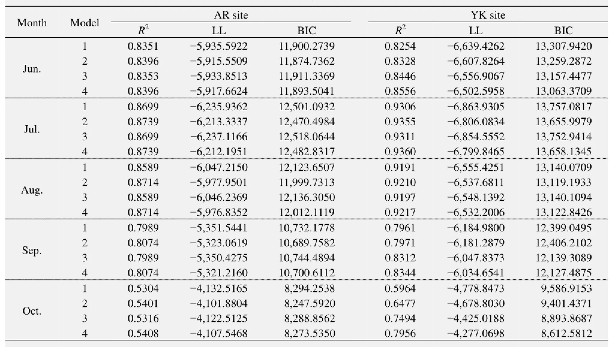
Table S1 Evaluation the results during the growing season by four carbon flux models

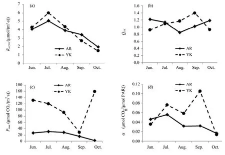
Figure S1 Seasonal patterns of parameter dynamics during the growing season by the Model 1 at AR and YK sites

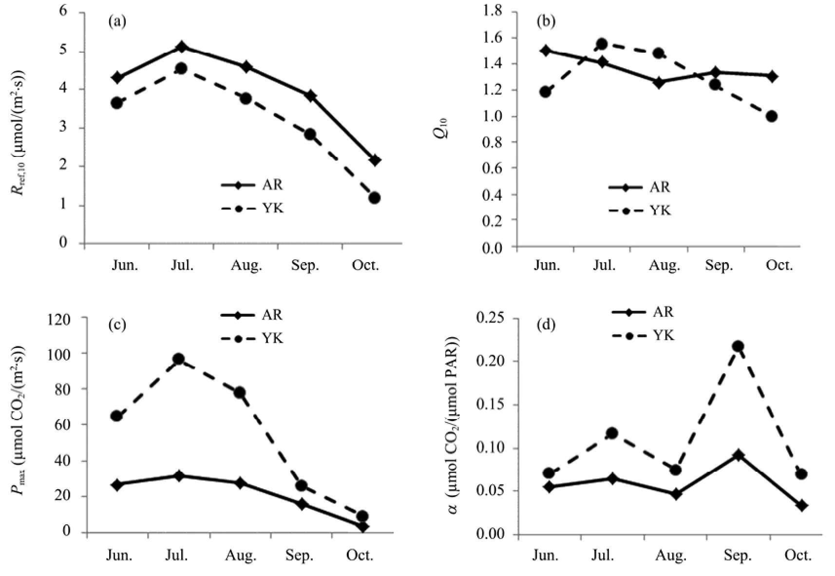
Figure S2 Seasonal patterns of parameter dynamics during the growing season by the Model 4 at AR and YK sites

Wang HB， Ma MG， 2015. Comparing the seasonal variation of parameter estimation of ecosystem carbon exchange between alpine meadow and cropland in Heihe River Basin， northwestern China. Sciences in Cold and Arid Regions， 7（3）： 0216-0228. DOI：10.3724/SP.J.1226.2015.00216.

*Correspondence to: Dr. HaiBo Wang, Assistant Professor of Cold and Arid Regions Environmental and Engineering Research Institute, Chinese Academy of Sciences. No. 320, West Donggang Road, Lanzhou, Gansu 730000, China. Tel: +86-931-4967972; E-mail: wanghaibokm@163.com

June 22, 2014 Accepted: February 10, 2015