LI Cheng-guang (李成光), XUE Wan-yun (薛万云), HUAI Wen-xin (槐文信)

State Key Laboratory of Water Resources and Hydropower Engineering Science, Wuhan University, Wuhan 430072, China, E-mail: licg@whu.edu.cn

Introduction

There are three main mixing processes in open channel flows: the molecular diffusion, the turbulent diffusion and the shear dispersion. Among them, the shear dispersion is the dominant mixing process, more important than others by several orders of magnitude.

The estimation of the dispersion coefficients has been a research focus for a long time. Marion et al.[1]discussed the effect of two contrasting mechanisms on the solute dispersion in meandering channels. Baek et al.[2]conducted flow and tracer experiments to study the mixing characteristics in a S-curved laboratory channel and it is found that the tracer cloud behaves quite differently depending on whether or not the tracer cloud is transported following the filament of the maximum velocity. Seo et al.[3]developed a 2-D advection-dispersion model with a heterogeneous dispersion coefficient tensor for meandering channels.Wilson et al.[4]used a 3-D model with the standardk-εturbulence closure to simulate the solute transport and mixing in a meandering self-formed channel and obtained a good fitting consistent with experiments. Etemad-Shahidi et al.[5]developed a M5’ Model Tree to predict the longitudinal dispersion coefficient in natural streams, which might be safely applicable in hydraulic and environmental studies.

The vegetation is ubiquitous in natural rivers.The effective water management requires a better understanding of the flow structures and the dispersion in vegetated channels. Most studies focused on the flow dynamics in vegetated channels[6-11], while studies of the dispersion coefficients in vegetated channels were relatively few. Ghisalberti and Nepf[12]conducted continuous dye experiments in a straight flume with a model vegetation to study the vertical mass transport in vegetated shear flows; it is shown that the coherent vortices of a vegetated shear layer dominate the vertical transport. Shucksmith et al.[13]presented a new data set quantifying the effect of the natural vegetation on the longitudinal mixing process in a straight flume.

Fig.1 Vegetation arrangements

So far, existing studies concern mainly the vegetation effects in straight channels, rather than meandering or strongly curved channels. Zhang et al.[14]presented a 2-Dk-εturbulence model for the curved open channel flow in curvilinear coordinates to simulate the hydrodynamic behavior of the turbulent flow in an open channel with a partial vegetation. Gorrick and Rodríguez[15]conducted laboratory experiments in a low-sinuosity, variable-width bend with and without vegetation on the outer bank, showing that the vegetation patches can greatly change the flow structures and force-balance components. In this paper, experiments are conducted to investigate the flow field in a 180ocurved vegetated flume. Based on the experimental data, the effect of the vegetation on the transverse and longitudinal dispersion coefficients is analyzed by using modifiedN-zone models.

1. Experimental setup

The experiment is conducted in a deep plexiglas flume of 14.28 m long, 1 m wide and 0.25 m high,with rectangular cross-section, consisting of a 4 m straight inflow reach, ao180 curved reach, and a 4 m straight outflow reach. The discharge is set to be 0.030 m3/s. Reinforcing steel bars are used to simulate the rigid vegetation of 0.006 m in diameter and 0.154 m in height. In this paper, two types of vegetation arrangements are discussed (as shown in Fig.1).The vegetation is in a parallel arrangement along the arc in both cases with the interval distance of 0.05 m.There is also a base case with no vegetation (as shown in Table 1). The 3-D acoustic Doppler anemometer(ADV) is used to measure the velocities on 5 typical cross-sections with 8 verticals for each cross-section and 7-8 measuring points for each vertical as needed.The sampling time is set to 60s to ensure the accuracy and reliability with the frequency of 50 Hz.

2. Flow field

Figure 2 and Fig.3 show the depth-averaged velocity distributions and the velocity vectors in the upper part of the flume (h=0.135m)on 5 typical cross-sections for the two vegetation cases. It can be seen that velocity is redistributed due to the existence of vegetation in both cases. Under the delayed effect of the vegetation, the velocities in the vegetation area are much smaller than those in the non-vegetation area.A large velocity gradient is generated between the vegetation area and the non-vegetation area, indicating that there must be remarkable mass and momentum exchanges at the junction of these two areas, which can also be verified from the secondary currents in Fig.4. In both vegetated cases, the secondary currents are confined to the non-vegetation area, and no evident circulation is generated in vegetation areas.

3. Dispersion coefficients

3.1 Transverse dispersion coefficient

Chikwendu[16]presented a model for calculating the longitudinal dispersion coefficient of laminar or turbulent 2-D channel or pipe flows, where the primary velocities were divided intoNseparate zones vertically to calculate the longitudinal dispersion coefficient, respectively. Boxall and Guymer[17]modified this model and applied it to calculate the transverse coefficient by dividing the transverse velocities intoNseparate zones vertically, assuming a full mixingin each zone (Fig.5). The transverse velocity here means the one that is perpendicular to the axis of the curve. The equations are expressed as

Table 1 Parameters of the experiment

Fig.2 Depth-averaged velocity distributions for different vegetation cases on 5 cross-sections

whereαjis water depth ratio of zonej.is themean transverse velocity in the firstjzones.is the mean transverse velocity in the lastN-jzones.is the interzone mixing coefficient between zonejand zonej+1, according to Boxall and Guymer[17],in curved channels.is transverse diffusion coefficient in zonej, andis the divided zone number, and hereN=7.

Fig.3 Velocity vectors in the upper part of the flume (h=0.135m) for different vegetation cases on 5 cross-sections

Figure 6 shows the calculated transverse dispersion coefficients using the modifiedN-zone model along the curved reach in these three cases. Compared with the base case, the transverse dispersion coefficients in both vegetation cases differ only a little. It can be seen that the vegetation has relatively small effect on the transverse dispersion. The possible reason may be that the delayed effect of the vegetation (decreasing the transverse dispersion coefficient) counteracts the velocity gradients generated between the vegetation area and the non-vegetation area (increasing the transverse dispersion coefficient) in general. In addition,the maximum value occurs at the 90ocross-section without vegetation, indicating that here the secondary flow has the biggest strength and the lateral mixing is the most violent.

3.2 Longitudinal dispersion coefficient

Chikwendu[16]divided the primary velocities intoNseparate zones to calculate the longitudinal dispersion coefficient. However, the main velocity profile contributing to the longitudinal mixing in an open channel flow, mostly influenced by the natural channel features, is the transverse profile of the depth average primary velocities[18]. So in this paper,Chickwendu’ method is modified to divide the primary velocities intoNzones transversely to calculate the longitudinal dispersion coefficient, assuming a full mixing in each zone[18](Fig.7). The primary velocity here means the one that is parallel to the axis of the curve. The equations are as follows

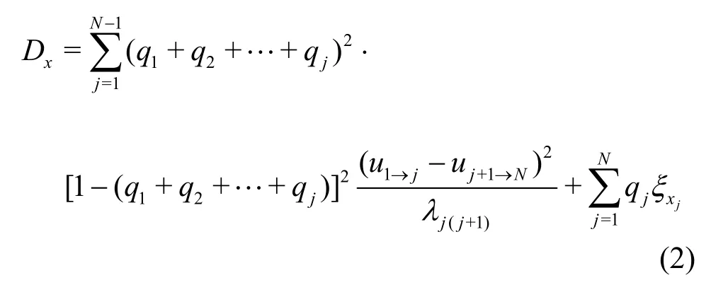
whereqjis water width ratio of zonej.u1→jis the depth-averaged velocity in the firstjzones.is the depth-averaged velocity in the lastN-jzones.is the interzone mixing coefficient between zonejand zonej+1, hereis equal tokyin the above expression,is longitudinal diffusion coefficient in zonej, andNis the divided zone number,and hereN=8.

Figure 8 shows the calculated longitudinal dispersion coefficients along the curved reach in 3 cases.It can be seen that the longitudinal dispersion coefficients in both vegetation cases are much larger than those in the base case. The maximum value reaches 0.93 m2/s as compared with the maximum value of 0.16 m2/s in the base case. The main reason may be that the flow velocities become much more inhomogeneous due to the presence of vegetation, which directly enhances the longitudinal dispersion. And also the

generation of the gradient exacerbates this trend. It can be concluded that the vegetation has a great effect on the longitudinal dispersion in the curved open channel flow.

Fig.4 Comparison of secondary flow structures for different cases on 2 typical cross-sections

Fig.5 Schematic diagram of modified N-zone model for calculating the transverse dispersion coefficient

Fig.6 Comparison of transverse dispersion coefficients along the curved reach for different cases

Fig.7 Schematic diagram of modified N-zone model for calculating the longitudinal dispersion coefficient

Fig.8 Comparison of longitudinal dispersion coefficients along the curved reach in different cases

4. Conclusions

The effect of vegetation on the flow structures and the dispersion in ao180 curved open channel is investigated with experiments and modifiedN-zone models. Main findings are as follows:

(1) Velocities in the vegetation area are much smaller than those in the non-vegetation area due to the presence of vegetation.

(2) A large velocity gradient is generated between the vegetation area and the non-vegetation area,indicating a remarkable mass and momentum exchange at the junction of these two areas.

(3) The vegetation has a relatively small effect on the transverse dispersion coefficient. However, since the primary velocities become much more inhomogeneous with the presence of vegetation, the longitudinal dispersion coefficients increase significantly.

[1] MARION A., ZARAMELLA M. Effects of velocity gradients and secondary flow on the dispersion of solutes in a meandering channel[J]. Journal of Hydraulic Engineering, ASCE, 2006, 132(12): 1295-1302.

[2] BAEK K. O., SEO I. W. and JEONG S. J. Evaluation of dispersion coefficients in meandering channels from transient tracer tests[J]. Journal of Hydraulic Engineering, ASCE, 2006, 132(10): 1021-1032.

[3] SEO I. W., LEE M. E. and BAEK K. O. 2D modeling of heterogeneous dispersion in meandering channels[J].Journal of Hydraulic Engineering, ASCE, 2008,134(2): 196-204.

[4] WILSON C., GUYMER I. and BOXALL J. B. et al.Three-dimensional numerical simulation of solute transport in a meandering self-formed river channel[J].Journal of Hydraulic Research, 2007, 45(5): 610-616.

[5] ETEMAD-SHAHIDI A., TAGHIPOUR M. Predicting longitudinal dispersion coefficient in natural streams using M5’ model tree[J]. Journal of Hydraulic Engineering, ASCE, 2012, 138(6): 542-554.

[6] JALONEN Johanna, JÄRVELÄ Juha. Estimation of drag forces caused by natural woody vegetation of different scales[J]. Journal of Hydrodynamics, 2014,26(4): 608-623.

[7] NEZU I., ONITSUKA K. Turbulent structures in partly vegetated open-channel flows with LDA and PIV measurements[J]. Journal of Hydraulic Research, 2001,39(6): 629-641.

[8] THOMPSON A. M., WILSON B. N. and HUSTRULID T. Instrumentation to measure drag on idealized vegetal elements in overland flow[J]. Transactions of the ASAE, 2003, 46(2): 295-302.

[9] STOESSER T., SALVADOR G. P. and RODI W. et al.Large eddy simulation of turbulent flow through submerged vegetation[J]. Transport in porous media, 2009,78(3): 347-365.

[10] NIKORA N., NIKORA V. and O’DONOGHUE T. Velocity profiles in vegetated open-channel flows: Combined effects of multiple mechanisms[J]. Journal of Hydraulic Engineering, ASCE, 2013, 139(10): 1021-1032.

[11] HSIEH P. C., SHIU Y. S. Analytical solutions for water flow passing over a vegetal area[J]. Advances in Water Resources, 2006, 29(9): 1257-1266.

[12] GHISALBERTI M., NEPF H. Mass transport in vegetated shear flows[J]. Environmental Fluid Mechanics,2005, 5(6): 527-551.

[13] SHUCKSMITH J. D., BOXALL J. B. and GUYMER I.Effects of emergent and submerged natural vegetation on longitudinal mixing in open channel flow[J]. Water Resources Research, 2010, 46(4): 1-14.

[14] ZHANG Ming-liang, SHEN Yong-ming and ZHU Lanyan. Depth-averaged two-dimensional numerical simulation for curved open channels with vegetation[J].Journal of Hydraulic Engineering, 2008, 39(7): 794-800(in Chinese).

[15] GORRICK S., RODRÍGUEZ J. F. Flow and force-balance relations in a natural channel with bank vegetation[J]. Journal of Hydraulic Research, 2014, 56(2):1-17.

[16] CHIKWENDU S. C. Calculation of longitudinal shear dispersivity using anN-zone model asNyields infinity[J]. Journal of Fluid Mechanics, 1986, 167:19-30.

[17] BOXALL J. B., GUYMER I. Analysis and prediction of transverse mixing coefficients in natural channels[J].Journal of Hydraulic Engineering, ASCE, 2003,129(2): 129-139.

[18] BOXALL J. B., GUYMER I. Longitudinal mixing in meandering channels: New experimental data set and verification of a predictive technique[J]. Water Research, 2007, 41(2): 341-354.