LUO Xionglin (罗雄麟)**, LIU Yubo (刘雨波) and XU Feng (许锋)

Research Institute of Automation, China University of Petroleum, Beijing 102249, China

Interaction Analysis and Decomposition Principle for Control Structure Design of Large-scale Systems*

LUO Xionglin (罗雄麟)**, LIU Yubo (刘雨波) and XU Feng (许锋)

Research Institute of Automation, China University of Petroleum, Beijing 102249, China

Industrial processes are mostly large-scale systems with high order. They use fully centralized control strategy, the parameters of which are difficult to tune. In the design of large-scale systems, the decomposition according to the interaction between input and output variables is the first step and the basis for the selection of control structure. In this paper, the decomposition principle of processes in large-scale systems is proposed for the design of control structure. A new variable pairing method is presented, considering the steady-state information and dynamic response of large-scale system. By selecting threshold values, the related matrix can be transformed into the adjoining matrixes, which directly measure the couple among different loops. The optimal number of controllers can be obtained after decomposing the large-scale system. A practical example is used to demonstrate the validity and feasibility of the proposed interaction decomposition principle in process large-scale systems.

control structure, interaction analysis, interaction decomposition, threshold value

1 INTRODUCTION

In practical chemical processes, many alternatives are usually available, ranging from a fully centralized system to a fully decentralized one. If the fully centralized control method is adopted, the burden of calculation will be aggravated because of the high dimension of the process [1]. The internal interaction in the system is ignored, and it is difficult to tune the parameters [2, 3]. However, for the fully decentralized control system, which includes many single variable proportion-integral-derivative (PID) controllers, it is difficult to achieve a reasonable control performance because of the strong interactions among control loops. To solve this problem, the block decentralized control strategy, which lies between these two extreme control structures, is required. Decomposition, considering the interaction among the control loops, can provide the criterion to control structure selection. Thus research on the interaction analysis and interaction decomposition of large-scale systems is necessary.

The relative gain array (RGA) [4] based techniques has many important advantages, such as simplicity of calculation, as it only uses the steady-state gain matrix of the process. However, using steady-state gain alone may result in erroneous interaction measures and loop-pairing decisions. To overcome the limitations of RGA based on the loop-pairing criterion, several paring methods have been proposed by considering both steady-state and transient information of the process. For the dynamic relative gain array (DRGA) method [5], a proportional output optimal controller is designed based on the state space approach, and the resulting controller gain matrix is used to define the matrix using the available dynamic process model. However, DRGA is often controller dependent, making it more difficult to calculate and to be understood by practical control engineers. To combine the advantages of both RGA and DRGA, an effective relative energy array (ERGA) [6] based loop-pairing criterion is defined by employing the steady-state gain and bandwidth of the process transfer function element in the frequency domain. Although ERGA considers both steady-state and transient information of the process, its calculation depends on the bandwidth selection of the process without considering time delay. To address this disadvantage of ERGA, He et al. [7] introduced a relative normalized gain array (RNGA) based loop-pairing criterion by considering the steady-state gain and average residence time (AST) of the process in the time domain. As RNGA considers both steady-state gain and dynamic response, it provides a more comprehensive description of loop interactions. However, AST only focuses on the sum of the time constant and the time delay and it never considers the influence of time delay when the average residence time is constant. Ren et al. [8] introduced the relative energy gain array (REGA) method, which can balance the relationship between time constant and time delay. REGA is controller independent and is more superior to other existing loop-pairing methods. It will be introduced in Section 3.

Some researchers have conducted studies on loop decomposition-based interaction analysis. Zhu and Jutan [9] presented a method to decompose a system into several single-input single-output control loops with relative interactions. Similarly, Cai et al. [10] determined the gain and phase changes of a transfer function with other loops closed by employing the concept of integrated error. Based on the equivalent transfer function, the parameters of a stable, proper, and causal ideal diagonal decoupler can be easilydetermined by proper parameter assignments of the decoupled transfer function matrix elements. Although these two methods can be effectively used in a two-dimensional system, they are difficult to apply in high-dimension systems. To solve the problem of decomposing high-dimension systems, some new interaction decomposition methods have been published. Mario and Arthur [11] proposed a Gramian-based measure of the interaction in multivariable plants, which provides support for decentralized input-output pairing and for a rich controller architecture selection in continuous and discrete-time framework. Nevertheless, the decomposition result is not uniquely determined. Shen et al. [12] analyzed RNGA [7] to obtain an equivalent transfer function to decompose the multiple inputs and multiple outputs (MIMO) process control system and proposed a sparse control structure to provide a compromise between system performance and structural complexity. However, the sparse control structure is very complex. By defining a relative control performance index, RGA can be transferred to a relative gain array that can be decomposed [13]. A CH diagram is proposed to measure the interaction of control loops and to facilitate the control structure selection process. The RGA based loop-pairing criterion ignores the transient information of process, and it may lead to incorrect pairing results. Drawing the CH diagram of high-dimension systems is very complicated, and the method can not achieve the unique interaction decomposition.

Although some of these proposed techniques may satisfy control structure selection, no systematic method is available for control structure selection. Thus this paper intends to examine interaction analysis and interaction decomposition in large-scale system to design control systems. A new interaction analysis method based on the transfer function matrix of open loop, REGA, is introduced, which considers both the steady-state gain and the transient information of the process. REGA is then transferred into adjoining matrixes by selecting different threshold values. As the number of the threshold value increases, the number of optimal controller, Nopt, will be determined after decomposing the large-scale system. Two examples are presented to demonstrate that the proposed method is simple, effective, and easy to be implemented.

2 PRELIMINARIES

Considering an n×n system with multivariable feedback control structure as shown in Fig. 1, wheresystem; C(s) is the transfer function matrix of multivariable controller to be selected from all types of controllers ranging from full decentralized controllers to centralized controllers including block diagonal controllers; and r, u and y are vectors of references, manipulated and controlled variables respectively.

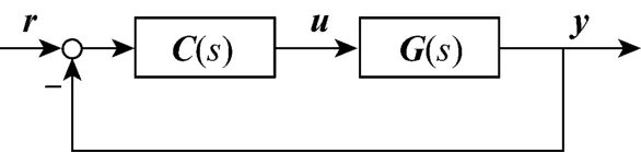
Figure 1 Block diagram of general multivariable control system

The relative gain for the variable pairing yi-ujis defined as the ratio of two gains representing the process gain in an isolated loop and the apparent process gain in the same loop when all others loopsRGA, ()ΛG, in matrix form, is defined as,the Hadamard product andT−G is the transpose of the inverse of G.

One of the main advantages of this pairing rule is that the interaction evaluation depends on the steadystate gains only. However, this pairing method may result in wrong interaction measures and loop-pairing decisions. To overcome the limitation of RGA based loop pairing criterion, the loop pairing methods combining with steady state information and transient character are developed. The ERGA considers the steady state gain and bandwidth of the process transfer function element. However, since the calculation of ERGA depends on the critical frequency point of individual element, different section criteria for critical frequency points will result in different ERGAs. To improve the ERGA, the RNGA based loop-pairing criterion can consider both steady-state and transient information in the time domain. RNGA, Φ, in matrixis the average residence time which is the sum of the time constant and time delay. It never considers the effect of time delay for variable pairing when the average residence time is constant. The following example is provided as an illustration.

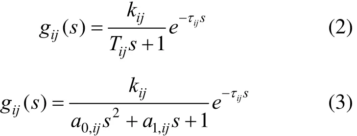
Example 1 Consider a 2×2 process with the transfer function matrix [8]:

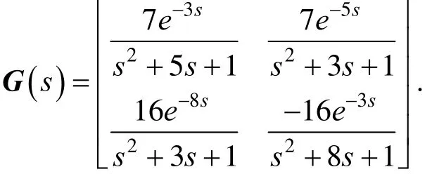
The steady-state RGA and RNGA are obtained as

The RGA and RNGA matrixes can not determine the pairing result. RGA uses the steady-state gain alone and can not consider the dynamic property of the process. Although RNGA considers both the steady-state and dynamic information of the process, it never takes time delay into account. Thus a reasonable variable pairing can be obtained only if the time constant and time delay can be perfectly balanced.

3 INTERACTION ANALYSIS FOR LARGESCALE SYSTEMS

Variable pairing is an important step in the design of the process control system [14]. The time delay is always present in practical systems, and its level plays an important role in control performance and variable pairing. This paper presents a variable pairing method, REGA, which can balance the relationship between the time delay and the time constant.

3.1 The index of energy consumption

Suppose that a system dynamic model is available and that the transfer function matrix of the controlled system is in the following form [15],

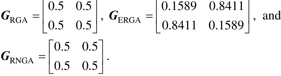
Without loss of generality, let each element of the process transfer function matrix be represented by the first order plus delay time (FOPDT) model and the second order plus delay time (SOPDT) model, both of which can describe most industrial processes.

where k is the proportionality coefficient, τ is the delay time, T is the time constant of FOPDT and a0, a1is the first coefficient and second coefficient of FOPDT.

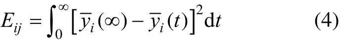
which represents the value of energy consumption [8].

For the common FOPDT and SOPDT, the following equations can be derived from Eqs. (2)-(4):

3.2 The relative energy gain array

For a MIMO system, interaction analysis of the control loops should consider steady-state gain and transient information. The transient character of REGA is measured by the value of energy consumption. Apparently, a small energy consumption value implies a fast dynamic response of the transfer function weak interaction from other loops, whereas a larger value indicates a slow dynamic response and severe coupling with other control loops.

Energy gain kE,ijis defined using the steady-state gain and the energy consumption value in REGA.

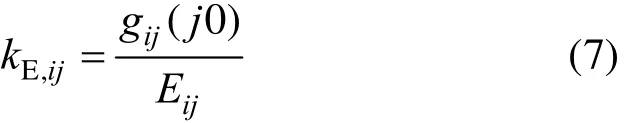
where gij(j0) is the steady-state gain and Eijis the energy consumption value.

Extending Eq. (7) to all elements of the transfer function matrix G(s), the energy gain matrix KEcan be obtained.

where ⊙ indicates an element-by-element division,

Similar to the definition of RGA, the steady-state gain matrix is replaced by the energy gain matrix KEin Eq. (8), and the relative energy gain (REG) between output variable yiand input variable ujis defined.

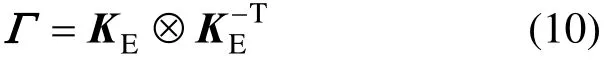
whereE,ijk′ is the energy gain between output variable yiand input variable ujwhen all other loops are closed. Hence, REGA can be calculated by the following equation

Similar to RGA based pairing rules, the REGA based loop pairing rules require that manipulated and controlled variables in a process control system should be paired.

(1) Corresponding REGA elements are closed to 1.0.

(2) All paired REGA elements must be positive.

(3) Large REGA elements should be avoided.

Example 1 Continue

REGA can be obtained through Eq. (10).

Reference [8] demonstrates that the diagonal pairing is the best one with the smallest interactions between control loops. The RGA only considers the steady state information so that it can not give a reasonable variable pairing result. Although the ERGA can consider steady-state and transient information, the calculation of ERGA is related to the selection of bandwidth without considering the time delay in frequency domain. In time domain, RNGA can not give a reasonable pairing criterion while time delay is very large and AST is constant. However, when the time delay is small and less than the time constant, the loop pairing result from REGA is same to that from RNGA. That is to say, the REGA can make up the deficiency of the RNGA.

4 INTERACTION DECOMPOSITION PRINCIPLE FOR LARGE-SCALE SYSTEMS

For an n×n process control system, the control loop interaction can be classified into two extreme situations. (1) When the interaction among control loops is weak, the control system can be designed as n single variable controllers. (2) When the interaction among the control loops is strong, the centralized control scheme is applied to the control system (i.e., only one PID controller). In practical process systems, the controller number must be selected from 1 to n. Considering the interaction, the minimum number of the overall controllers Nmin(Nmin≥1) should be obtained for large-scale systems with relatively strong interactions. For others with relatively weak interactions, the control system will contain the maximum controller number Nmax(Nmax≤n).

For a MIMO system, without interactions in some controlled objects that can be controlled by the conventional single-variable PID controller, it should not be decomposed. However, interaction decomposition should be used for some controlled objects with a strong couple among the control loops. After decomposing the MIMO system, some subsystems can still be controlled by the single-variable PID controller, such as REGA element close to 1, and then several 1×1 control subsystems can be determined. Some other subsystems can be controlled by multivariable PID controllers, such as REGA elements close to 0.5, and then several multivariable control subsystems can be obtained. The following example is used as a demonstration.

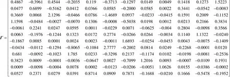
Example 2 Consider a 4×4 process with the following transfer function matrix:

In matrix Γ, the REGA elements indicate that the control loops y1-u1and y2-u2have weak interaction with other loops, which can be designed into 1×1 subsystems controlled by a single-variable PID controller. Control loops y3-u3and y4-u4present severe couple with other loops, which should not be decomposed, and they form a multivariable control system controlled by a multivariable PID controller. For a large-scale system, the number of controllers is directly related to the design cost and reliability of the control system.

Through the interaction decomposition principle presented in this paper, the upper limit Nmaxand the lower limit Nminof the controller number can be obtained after analyzing the interaction among the loops and selecting the same threshold value. The controller number is derived from the adjoining matrix, which can be calculated using REGA. According to the second paragraph in this section, the following two definitions of the adjoining matrix can be defined.

Definition 1 The elements in the adjoining matrix R=[γij]n×n, which can determine the lower limit Nminof the controller number, should be calculated according to the following criterion

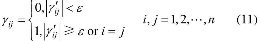
where γi′jrepresents the elements after adjusting the corresponding variables-pairing elements in REGA to the diagonal, and ε is the threshold value.

Definition 2 The elements in the adjoining matrix Q=[qij]n×n, which can determine the upper limit Nmaxof the controller number, should be calculated according to the following criterion

where γi′jrepresents the elements after adjusting the corresponding variables pairing-elements in REGA to the diagonal.

According to Definition 1, if all the elements γi′jare more than the threshold value, the elements in matrix R will be 1. Then, the controller number can be decided to be 1 and it is the minimum number of the controller, Nmin. As the selected threshold value increases, the elements in matrix R, 1, will decrease. Thus the lower limit Nminwill increase. As we know, when the elements in REGA are closed to 0.5, the couple among loops is the strongest. According to Definition 2, ifis more than the threshold value, the off-diagonal elements in matrix Q will be 0. Then, the controller number can be decided to be n. The upper limit Nmaxcan be obtained. As the selected value is large, the value of Nmaxwill decrease. As the selected threshold value increases, the values of Nminand Nmaxwill be equal. Then, the optimal controller number is derived.

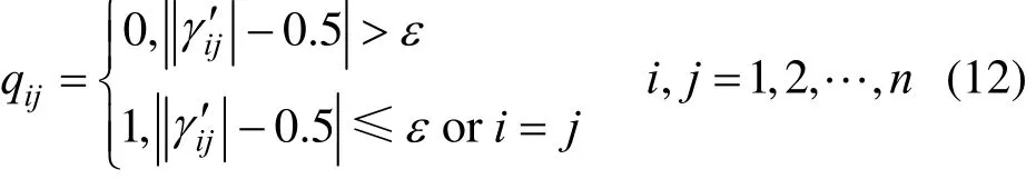
Remark 1 The range of the threshold value ε should be selected from 0 to 0.25. If the threshold value is larger than 0.25, 1s in R will decrease and 1s in Q will increase, resulting in Nmin>Nmax. Similarly, the range of seeking Nminand Nmaxwill overlap as the threshold value increases. Fig. 2 shows that the range ofijγ′ is selected as the threshold increases. When the threshold value ε is greater than 0.25, the interaction decomposition is the same as that when the threshold value ε is selected from 0 to 0.25. In other words, the value of the upper limit Nmaxwill be smaller than the lower limit Nmin. Then, the value of the upper limit Nmaxwill be the value of the minimum controller number. The largest threshold value is 0.25.

Figure 2 The range representations of value ′ijγ

5 ALGORITHM OF INTERACTION DECOMPOSITION

Based on the reasonable variable-pairing determined by REGA, two adjoining matrixes are determined by selecting the same threshold value ε. Then, Nminand Nmaxcan be determined. Finally, the optimal controller number Noptis obtained.

The algorithm for the interaction decomposition of large-scale systems is as follows.

Step 1 Calculate REGA by Eq. (9) and all the paired REGA elements must be positive and closest to 1.0 to obtain the best variable pairing.

Step 2 Exchange the places of the rows or ranks where the selected paired elements locate, such that the elements for the pairing of input and output are along the diagonal.

Step 3 Select the threshold value ε (0≤ε≤0.25) and determine the adjoining matrixes R and Q by Eqs. (10) and (11).

Step 4 Determine Nminand Nmaxfrom the adjoining matrix obtained in Step 3. If Nminis not equal to Nmax, increase ε and go to Step 3.

Step 5 Obtain the optimal controller number Nopt.

The following example demonstrates the algorithm of interaction decomposition.

Example 3 Consider a 4×4 process [16] with the following transfer function matrix:

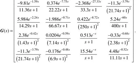
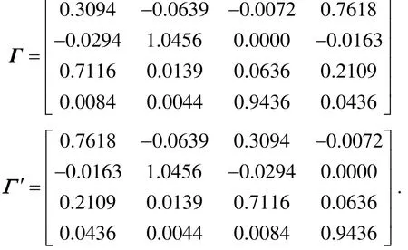
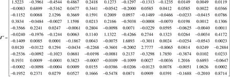
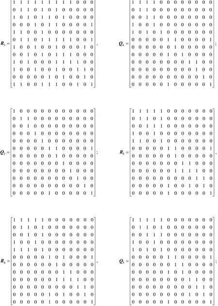
Calculating REGA and re-arranging the places for the pairing of input and output along the diagonal, the following matrixes are obtained:

Selecting the threshold values ε=0.05, 0.1, 0.15 and 0.2, the following adjoining matrixes are obtained, respectively,

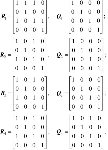
A series of controller numbers from the above matrixes can be determined. Fig. 3 shows the tendency of the controller number as the threshold value increases.

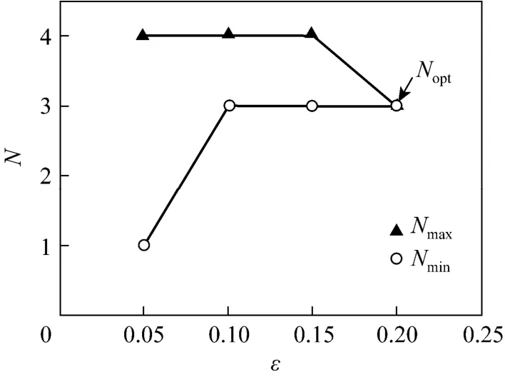
Figure 3 The tendency of controller numbers

Figure 3 shows three kinds of decomposition results for Example 3: only one controller (centralized control structure), four controllers (decentralized control structure) and three controllers (block decentralized control structure). The decentralized control structure is the pairing {(y1-u4), (y2-u2), (y3-u1), (y4-u3)}, and the block decentralized control structure is {(y1, y3)-(u4, u1), (y2-u2), (y4-u3)}. Applying with the RGA and ERGA and decomposing the control system, we can get the control structure that is {(y1-u4), (y2-u2), (y3-u1), (y4-u3)}. Thus the number of optimal controller derived by RGA and ERGA is 4. The result of decomposing the control system through the RNGA is the same to REGA. To compare the control performance of these three control structures, PID controllers are designed based on the internal model control (IMC) controller tuning rules [17, 18]. Fig. 4 compares the simulation results.

The control structure of the three PID controllers is optimal from the results of the simulation. The control structure of only one controller ignores the inner interaction of the system, and it is very difficult to tune its controller parameters. The control structure of the four subsystems controlled by four PID controllers does not consider the strong interaction among the control loops. We can say that the RGA and ERGA can not give a reasonable loop pairing criterion and the correct decomposing result. Hence, the use of the loop pairing method REGA and the interaction decomposition principle of large-scale system to achieve perfect control performance are significant. Example 3 demonstrates the effectiveness and necessity of the interaction analysis and interaction decomposition.

6 CASE STUDY: TENNESSEE EASTMAN PROCESS

The Tennessee Eastman (TE) plant-wide control system, developed by Downs and Vogel [19], has served as a useful vehicle for testing control strategies developed by different investigators. The authors have put multivariable control, on-line optimization, predictive control, identification and process diagnostics as potential applications. The TE process consists of five major unit operations: reactor, product condenser, vaporliquid separator, recycle compressor and product stripper. The details of the process can be found in Ref. [19].

The TE process involves 41 measurements and 12 manipulated variables. From the design experience, eight flow and two temperature cascade loops can be closed [20]. The flow loops include four feed streams: purge stream, stripper bottoms, separator bottoms and stripper steam flow. The two temperature cascades include the condenser and reactor cooling streams, as analyzers are typically less reliable than the more common temperature, pressure, flow, and level sensors. Analyzer loops are also typically slower. Thus 19 analyzer measurements are eliminated, then there are 41−10−19=12 potential variable to be controlled.Those controlled and manipulated variables are listed in Table 1. Since the dynamic model of the TE process is available, the transfer function matrixes of the process are identified using the Matlab identification toolbox [21, 22]. The identification results are listed in Appendix Table A1.

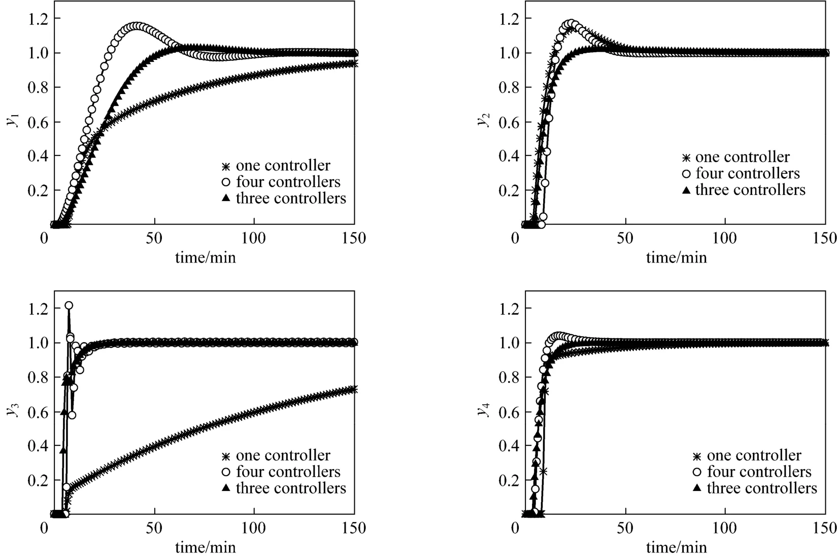
Figure 4 The results of simulation comparison for Example 3

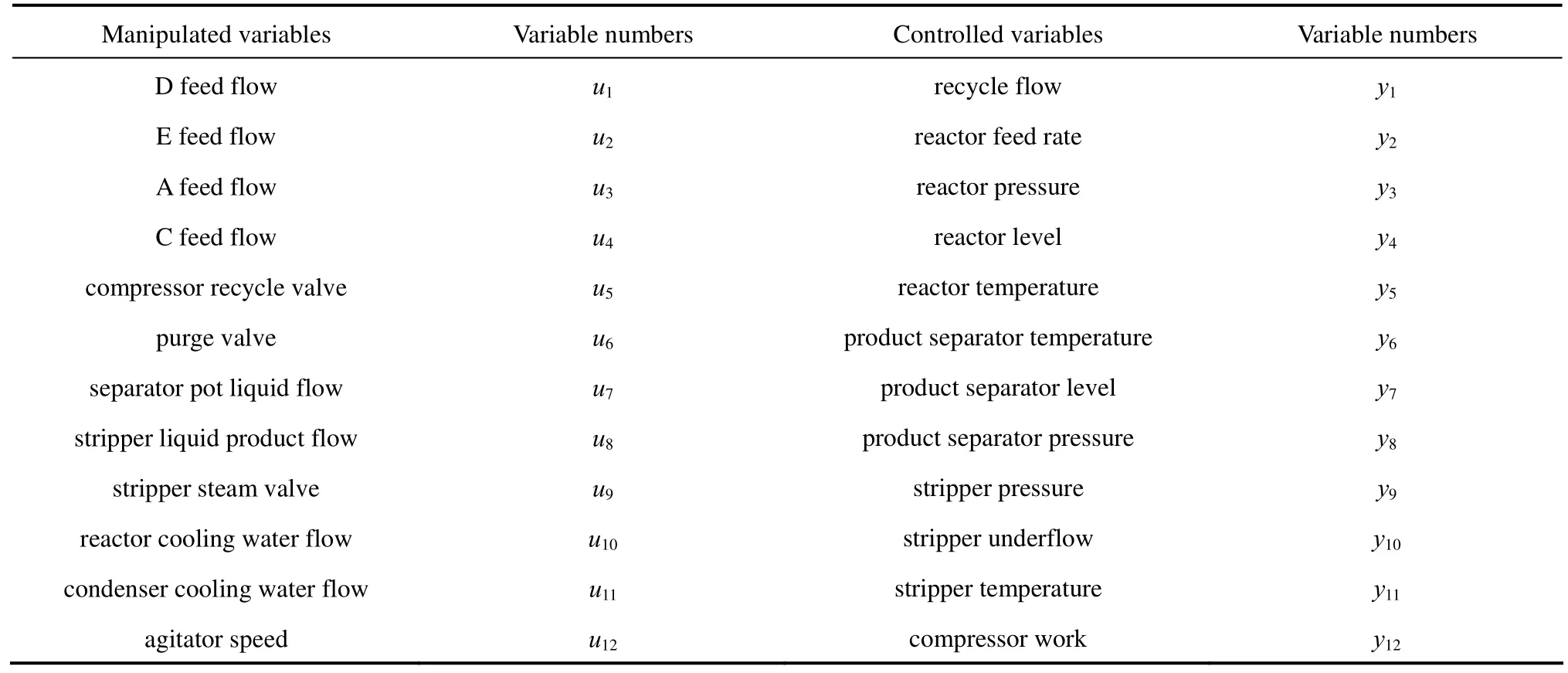
Table 1 Manipulated variables and controlled variables

In practical chemical processes, the derivation of subsystems is judged by the physical location. The TE process can be decomposed into three subsystems, reaction system, separation system and stripper system [23]. The decomposition result is in accord with engineers’ experience. Fig. 5 shows the three subsystems for the TE process.

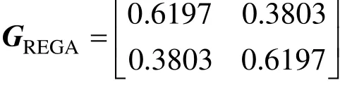
Although some proposed techniques may satisfy control structure selection, no systematic and theoretic method is applicable to the control structure selection. The interaction analysis and interaction decomposition proposed in this paper can make up the shortage in the control structure selection. Calculating REGA and re-arranging the places for the pairing of input and output along the diagonal, the following matrixes are obtained:

Figure 5 The result of decomposition for TE process1, A—feed A; 2, D—feed D; 3, E—feed E; 4, C—feed C; 5—stripper overhead; 6—reactor feed; 7—reactor product; 8—recycle; 9—purge;10—separation liquid; 11—product; CWS—cooling water supply; CWR—cooling water recycle; vap—vapour; liq—liquid; Stm—stream; Cond—condensate water; XA-XH—composition of A-H; FI—flow rate indicator; TI—temperature indicator; LI—level indicator; PI—pressure indicator; SC—safty controller

Selecting the threshold values ε=0.002, 0.05, 0.1, 0.15, 0.2 and 0.23, the following adjoining matrixes are determined, respectively,

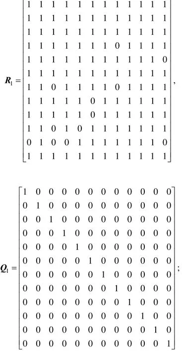
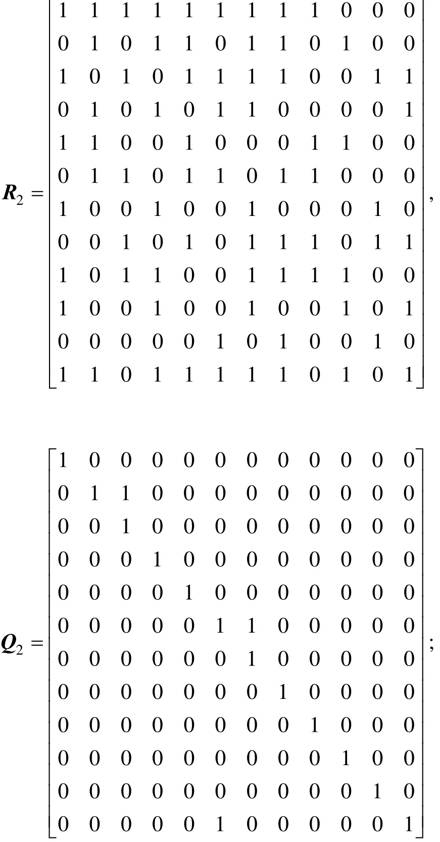
The number of controllers for the TE process can be determined by calculating these matrixes. Fig. 6 shows the tendency of the controller number as the threshold value increases.

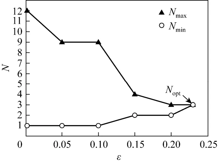
Figure 6 The tendency of controller numbers for the TE process

With the interaction decomposition principle applied to the TE process, adjoining matrixes R6and Q6indicate that the optimal controller number is 3, when Nmax=Nmin, indicating that the TE plant can be decomposed into three subsystems, namely, (y1, y2, y3, y4, y5)-(u12, u2, u3, u1, u10), (y6, y7, y8, y12)-(u11, u7, u6, u5) and (y9, y10, y11)-(u4, u8, u9). Result of the decomposition shows that the sites of the three subsystems are consistent with the physical place of the TE plant, according to the decomposition of the practical control system design. Result of the interaction decomposition for the TE plant demonstrates that the interaction decomposition proposed in the present paper is useful in practice and it can server as a guideline for practical control structure design. Fig. 5 shows the results of the interaction decomposition and the practical decomposition for the TE process.

7 CONCLUSIONS

The paper aims to determine the optimal controller number by decomposing large-scale systems. From the perspective of control system design, a new variable pairing is introduced to consider both steady-state and transient information, and the interaction decomposition principle for the large-scale systems is proposed. By selecting the threshold value, REGA is transferred into two adjoining matrixes, which can measure the interaction relationship between the input variables and output variables, and determine the upper limit Nmaxand the lower limit Nmin. As the threshold value increases, the value Nmaxwill equal Nmin. At this point, the optimal controller number Noptis determined. By analyzing the TE plant, the validity and feasibility of interaction decomposition are illustrated.

REFERENCES

1 Foss, A.S., “Critique of chemical process control theory”, AIChE J, 19 (2), 209-214 (1973).

2 Wang, Q.G., Huang, B., Guo, X., “Auto-tuning of TITO decoupling controllers from step tests”, ISA Transactions, 39 (4), 407-418 (2000).

3 Tavakoli, S., Griffin, I., Fleming, P.J., “Tuning of decentralized PI (PID) controllers for TITO processes”, Control Engineering Practice, 14 (9), 1069-1080 (2006).

4 Bristol, E.H., “On a new measure of interaction for multivariable process control”, IEEE Transactions on Automatic control, 11 (1), 133-134 (1966).

5 McAvoy, T.M., Arkun, Y., Chen, R., Robinson, D., Schnelle, P.D., “A new approach to defining a dynamic relative gain”, Control Eng. Practice, 11 (8), 907-914 (2003).

6 Naini, N.M., Fatehi, A., Sedigh, A.K., “Input-output pairing using effective relative energy array”, Ind. Eng. Chem. Res, 48 (15), 7137-7144 (2009).

7 He, M.J., Cai, W.J., Ni, W., Xie, L.H., “RNGA based control system configuration for multivariable processes”, Journal of Process Control, 19 (6), 1036-1042 (2009).

8 Ren, L.H., Liu, Y.B., Luo, X.L., Xu, F., “Interaction analysis and variable paring for multivariable system with time delays”, Control and Instruments in Chemical Industry, 39 (6), 743-746 (2012).

9 Zhu, Z.X., Jutan, A., “Loop decomposition and dynamic interaction analysis of decentralized control systems”, Chemical Engineering Science, 51 (12), 3325-3335 (1996).

10 Cai, W.J., Ni, W., He, M.J., Ni, C.Y., “Normalized decoupling—A new approach for MIMO process control system design”, Ind. Eng. Chen. Res., 47 (19), 7347-7356 (2008).

11 Mario, E.S., Arthur, C., “MIMO interaction measure and controller structure selection”, INT. J. Control, 77 (4), 367-383 (2004).

12 Shen, Y.L., Cai, W.J., Li, S.Y., “Multivariable process control: decentralized, decoupling, or sparse”, Ind. Eng. Chen. Res., 49 (2), 761-771 (2010).

13 He, M.J., Cai, W.J., Wu, B.F., “Block control structure selection based on relative interaction decomposition”, In: 9th International Conference on Control, Automation, Robotics and Vision, International Academic Publishers, Singapore, 1-6 (2006).

14 Ye, L.J., Song, Z.H., “Variable pairing method for multivariable control systems”, Control and Decision, 12 (6), 1795-1800 (2009).

15 Luo, X.L., Wang, H.Q., Xu, F., “Auxiliary regulatory control design of multivariable system in industrial process”, Control and Instruments in Chemical Industry, 36 (4), 33-37 (2009).

16 Luyben, W.L., “Simple method for tuning SISO controllers in multivariable systems”, Ind. Eng. Chem. Process Des. Dev, 25 (3), 654-660 (1986).

17 Astrom, K.J., Hagglund, T.H., PID Controllers: Theory, Design and Tuning, 2nd edition, Instrument Society of American, American (1995).

18 Hu, B., Zheng, P.Y., Liang, J., “Multi-loop internal model controller design based on a dynamic PLS framework”, Chin. J. Chem. Eng., 18 (2), 277-285 (2010).

19 Downs, J., Vogel, E., “A plant-wide industrial process control problem”, Computers and Chemical Engineering, 17 (3), 245-255 (1993). 20 McAvoy, T.J., Ye, N., “Base control for the Tennessee Eastman problem”, Computers and Chemical Engineering, 18 (5), 383-413 (1994).

21 Fang, C.Z., Xiao, D.Y., Process Identification, Tsinghua University Press, Beijing (1988).

22 Liu, S.J., Gai, X.H., Fan, J., Cui, S.L., MATLAB 7.0 Control System Application and Example, China Machine Press, Beijing (2006).

23 Tian, Z.H., Hoo, K., “Multiple model-based control of the Tennessee-Eastman process”, Ind. Eng. Chem. Res., 44 (9), 3187-3202 (2005).

APPENDIX

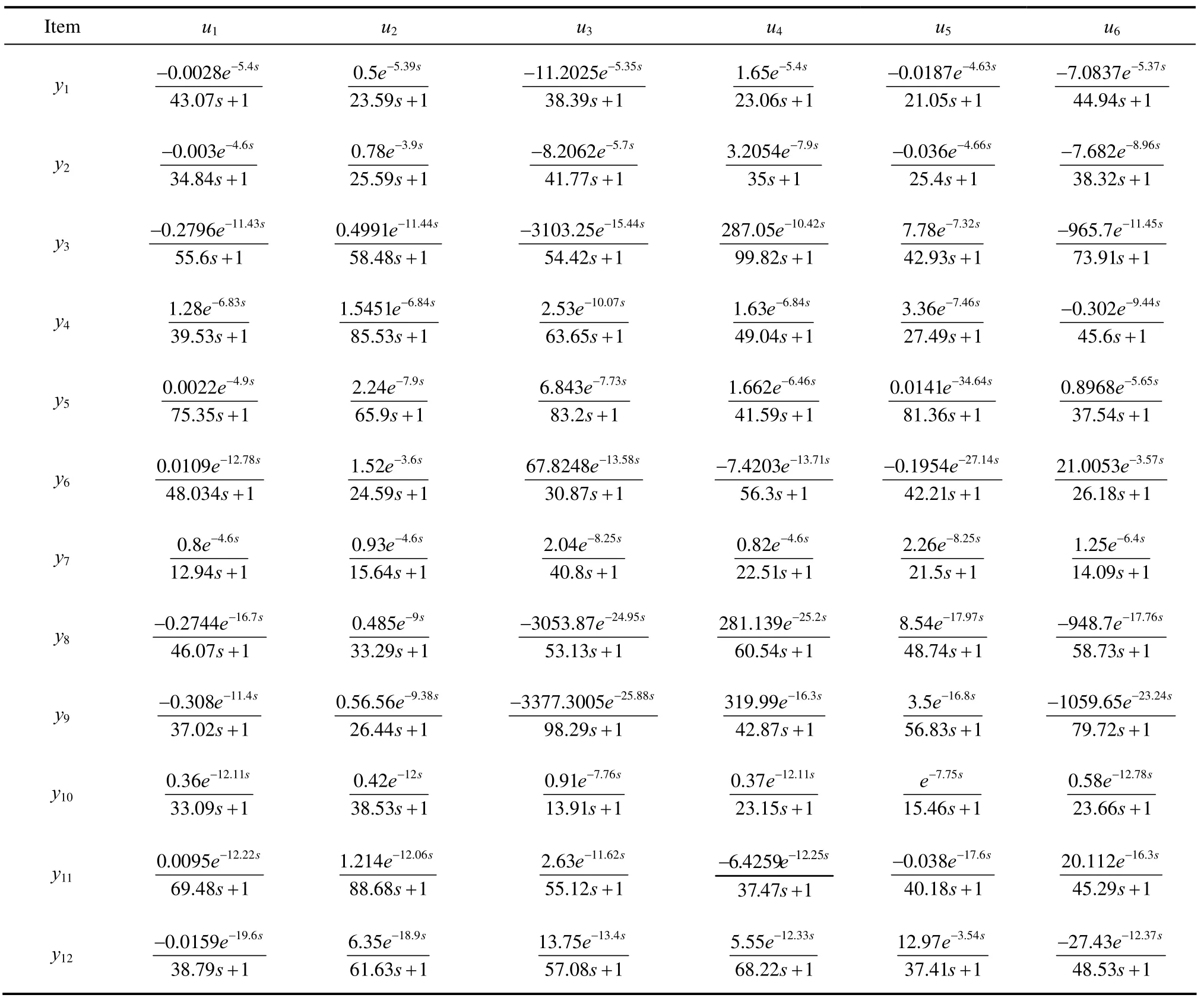
Table A1 Some transfer function matrixes of the TE process

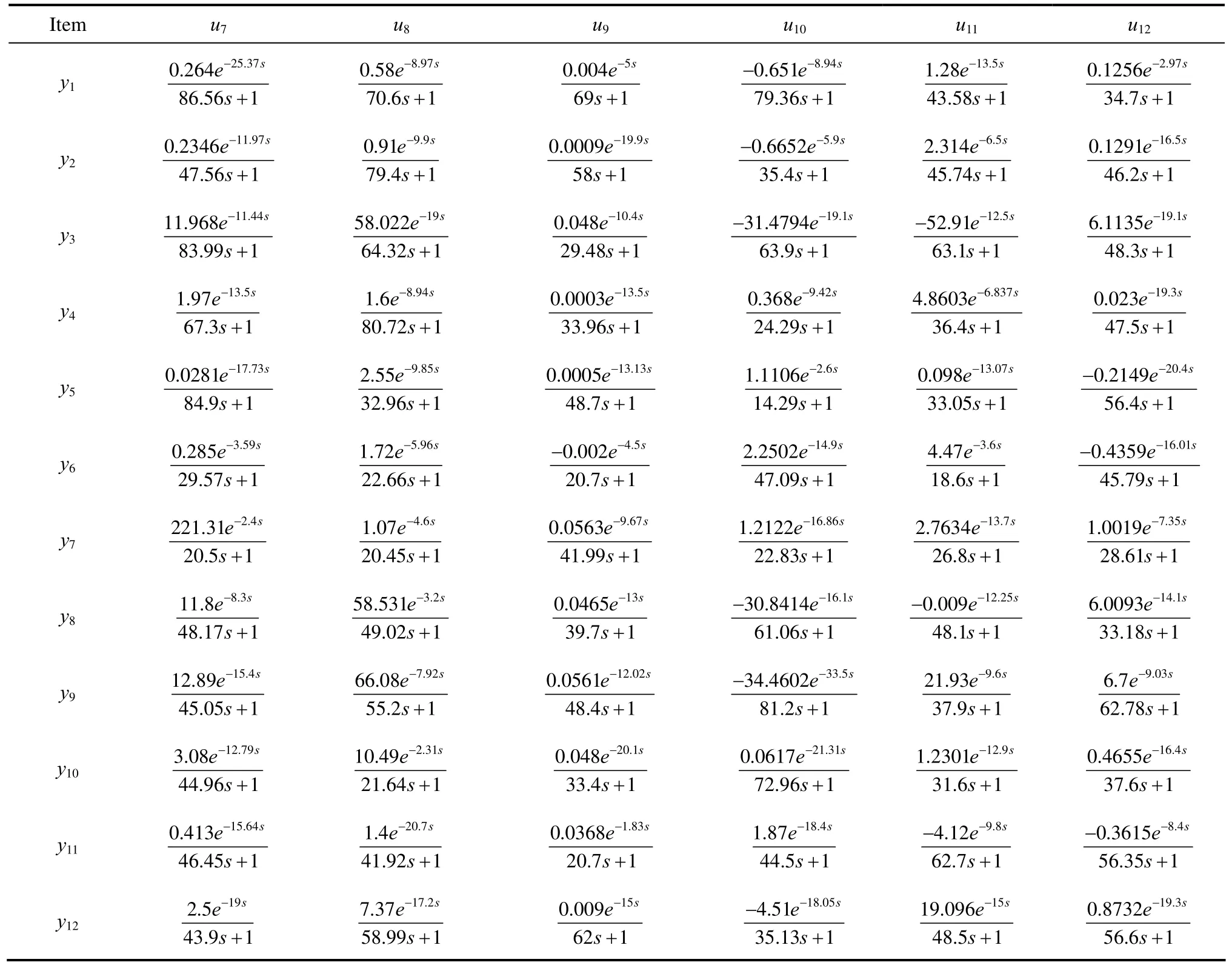
Table A1 (Continued)

10.1016/S1004-9541(14)60002-1

2013-03-04, accepted 2013-05-22.

* Supported by the National Natural Science Foundation of China (21006127) and the National Basic Research Program of China (2012CB720500).

** To whom correspondence should be addressed. E-mail: luoxl@cup.edu.cn