Sun Kaipeng（孙凯鹏），Hu Haiyan（胡海岩），Zhao Yonghui（赵永辉）

State Key Laboratory of Mechanics and Control of Mechanical Structures，Nanjing University of Aeronautics and Astronautics，Nanjing，210016，P.R.China

1 Introduction

Hypersonic flight vehicles are subject to very tough aerodynamic load and heating during their missions［1］.The aerodynamic heating produces adverse effects on the dynamic performance of a hypersonic flight vehicle，and even results in strong vibrations or dangerous flutters［2］.From the view point of structural dynamics of hypersonic flight vehicles，the severe aerodynamic heating not only reduces the mechanical properties，such as Young′s modulus，of any structural material，but also gives rise to the dangerous thermal stress in any constrained structural component.Hence，the heated structure in a hypersonic flight vehicle undergoes the change of structural stiffness in both quantity and distribution，as well as the change of modal parameters，with an increase of heating time.That is，the heated structure of a hypersonic flight vehicle is a time－varying system，which features the vibration modes with time－varying properties.

The studies on the dynamic analysis of thermo－elastic structures，such as beams and plates，under constant or time－varying temperature environment have been quite extensive［3－8］.For example，Avsec and Oblak studied how the temperature field had an impact on the vibration of beams and found that a small change of temperature might cause significant changes of natural frequencies of beams［4］.Xiao and Chen analyzed the buckling and vibration problems of a thin elastic－plastic square plate with four immovably simply－supported edges in a uniform temperature field［7］.Huang and Wang analyzed the modal of a variable－thickness plate under the transient thermal environment，and derived the modal parameters at different moments［8］.To the best knowledge of authors，the studies on the thermoelastic structure dynamics mainly focuse on the direct problems of analysis，instead of the inverse problems，such as system identification or input identification.

The time－varying vibration modes occur not only in the heated structure of a hypersonic flight vehicle in a real mission，but also in such a structure in a thermal－vibration test on ground.As a matter of fact，it is very difficult to keep a long steady heating for such a structure during the thermal test，especially in the case of extremely high temperature.It is thus necessary to deal with the time－varying modal problem of thermo－elastic structures.For model verification and heated structure validation，it is important to identify the time－varying vibration modes of a heated structure by its thermal－vibration measured in a ground test.

The dynamic identification and parameter estimation for a time－varying linear system are the forefront of the inverse problem in structural dynamics.Two major kinds of methods have been developed for such inverse problems.One is the time－frequency methods，such as the Gabor transform and wavelet transform［9－13］.The other is the time series methods，such as time－varying autoregressive（TVAR）method and time－varying autoregressive moving average（TVARMA）method［14－20］.Approaches for estimating the TVAR parameters can be classified into two categories，namely，the adaptive algorithm and the basis function method.Even though the adaptive algorithm can track the slowly time－varying frequency or the frequency jump efficiently，they are sensitive to measurement noise and initial conditions.They also fail to track the time－varying frequencies of a system in which frequencies change very fast or change in a wide range［16］.The basis function expansion and regression approach has the excellent capability of tracking time－varying system parameters［16，19－20］.However，the selection of expansion dimension is questionable since there is no theoretical criterion for the selection.

Recent attention has been paid to the practical problem for selecting order p of the autoregressive（AR）model and dimension m of the basis functions.Many criteria have been proposed because the problem of model selection arises frequently in regression analysis.Final prediction error（FPE）criterion，Akaike information criterion（AIC）and Bayesian information criterion（BIC）are the most popular methods for selecting orders［21－24］.However，the FPE，AIC and BIC functions are often not strictly concave down，and sometimes are accompanied by random fluctuations，in the actual process for selecting orders［24］.This problem may let the criterion function reach a certain value without any obviously changing trend，but oscillating up and down randomly，which sequentially affects the correctness and effectiveness of order selection.Furthermore，these methods cannot determine the dimension of basis functions，but only pick the order of the AR model.In this work，hence，a new method combined by BIC and grey correlation analysis（GCA）is developed to solve the problem of model selection and to determine the order and dimension concurrently.

The work focuses on the estimation of slowly time－varying modal parameters of a thermo－elastic structure with sparse natural frequencies，such as beams and panels frequently used in hypersonic flight vehicles.Here the"slowly"means that the time scale of the temperature variation is much larger than that of the thermo－elastic structure vibration，and thermal－induced oscillation do not occur.

2 Dynamic Equations of Thermo－Elastic Beams

2.1 Simply－supported beam with axially movable boundary

For simplicity，the thermo－elastic structure in this paper is a simply－supported Euler－Bernoulli beam with a constant rectangular cross－section，as shown in Fig.1，subject to a distributed excitation f（x，t）and a uniformly distributed temperature field T（x，t）≡T（t）.Let l be the length of beam，Athe cross－section area of beam，and Ithe cross－section moment of inertia of beam about the axis y－y.The ordinary simply－supported beam has two axially immovable boundaries，which constrain the axial thermal expansion of the beam and greatly reduce the critical buckling temperature of it.To remove this shortcoming，it is natural to let one boundary axially movable so that the axial thermal expansion can be released.To well model the real boundary in this case，it is better to add an axial spring at the movable boundary as shown in Fig.1.

As a result of thermal expansion，the axial thermal force Nxyields

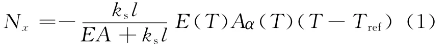
where ksis the stiffness coefficient of spring and minus sign means Nxis an axially compressive force.E（T）andα（T）are the Young′s modulus and the thermal expansion coefficient changing with temperature T，respectively.Trefis the reference temperature，i.e.，the room temperature.

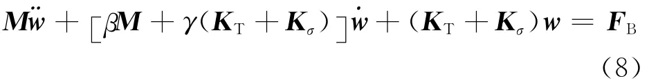
Using Hamilton′s principle，it is straightforward to establish the dynamic equation of the thermo－elastic beam as follows［4］

Substituting Eq.（1）into Eq.（2）gives the transverse dynamic equation of the beam as follows

2.2 Finite element formulation

Eq.（3）enables one to obtain the dynamic equation modeled by FEM in the following matrix form

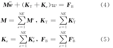
where the matrices of finite element are defined by the integrals

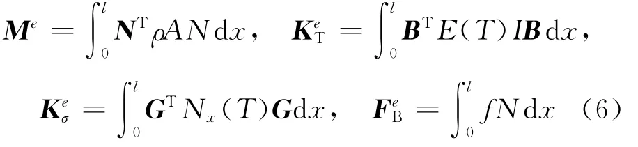
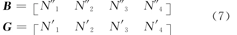
with the curvature interpolation matrix and the slope interpolation matrix as

The coefficient matrix Meis the element mass matrix andis the time－varying element stiffness matrix as a result of material performance degeneration due to heating.The coefficient matrixis the time－varying element stiffness matrix due to longitudinal load Nx（t）with the thermal effect.The load vectorrepresents the equivalent nodal loads due to the external force f.For simplicity，the proportional damping is used in this paper.Now，the dynamic equation with a temperature effect taken into account reads

3 Time－Varying Autoregressive Model

3.1 TVAR modeling and estimation

This subsection deals with a TVAR process（t）of order pin discrete－time as follows［14－15］

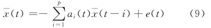
where e（t）is a stationary white noise process with zero mean and varianceσ2，and the TVAR coefficients｛ai（t），i＝1，2，…，p｝yield the following linear combination of a set of basis functions｛gj（t），j＝0，1，…，m｝

where aijare the weighted coefficients and mis the dimension of the basis functions.

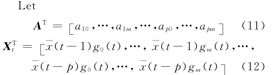
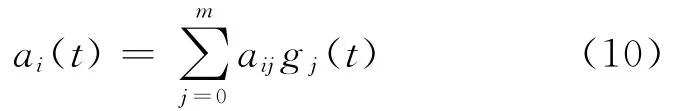
Then Eq.（9）can be expressed as

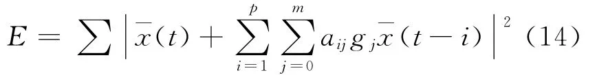
According to the principle of least square（LS），the estimation of｛aij｝aims at minimizing the total squared prediction error

Then，it is easy to get the LS estimate of｛aij｝

and the LS estimate of residual variance

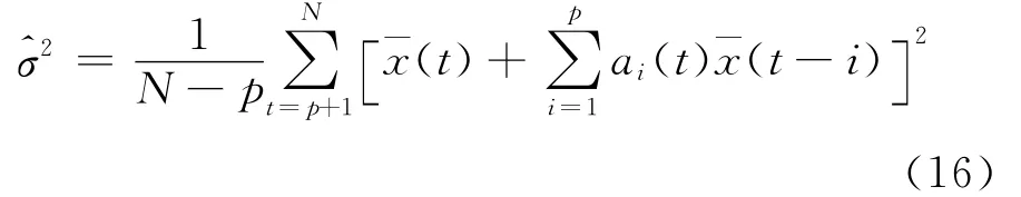
Eq.（15）shows that the LS estimate requires matrix inversion and may give rise to the problems of computational cost and storage space.In practice，it is appropriate to use the recursive least square（RLS）estimation based on the estimation of previous steps.

A variety of forgetting methods has been available so far to reduce the weight of the data in a distant past and reduce the effective memory of the RLS algorithm［25－26］.In this paper，the expo－nential forgetting method with a constant forgetting factor is used so that the parameter estimation algorithm can be written as

where the forgetting factorλis chosen in the interval（0，1］，and normally close to 1.The initial value of＾Aand Pcan be selected as＾A0＝0，P0＝μI，whereμ≥1and Iis the unit matrix.

3.2 Selection of order and dimension

The BIC of Akaike is the most popular method for selecting orders.As shown in Ref.［24］，the BIC can be expressed as

where Nis the number of the data samplings，＾σ the predicted error of the model and Ca constant larger than 1.When order pincreases，the firstitem of the right hand of Eq.（18）decreases，but the second item increases.The number p which minimizes the BIC value is regarded as the appropriate order.

As mentioned above in Introduction，there may be several local minima in FPE，AIC and BIC values.It is therefore difficult to pick the global minimum due to the fact that the FPE，AIC and BIC functions are often not strictly concave down，and sometimes are accompanied by random fluctuations，in the actual process for selecting orders.Furthermore，BIC can only pick the order of the AR model，but cannot determine the dimension of the basis functions.Hence，in this study，BIC is used to preliminarily determine the rough scope of order p.Then，order p and dimension m are determined simultaneously by using the theory of grey systems with the definition of absolute grey correlation degree（AGCD）.BIC thus reaches some minima so that the rough scope of the order number can be obtained preliminarily.After getting the scope of p，one can set up the range of dimension mas［0，8］for in－stance，and then build up the corresponding TVAR models.By means of the original LS estimator or RLS estimator，the AGCD between the TVAR model and the original signal｛｝can be acquired.The following steps give the definition and detailed algorithm for computing AGCD.

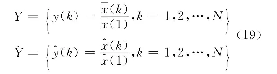
Step 1 Normalize the sequences X＝（k），k＝1，…，N ｝ and＝（k），k＝1，…，N ｝via their initial values.That is，let

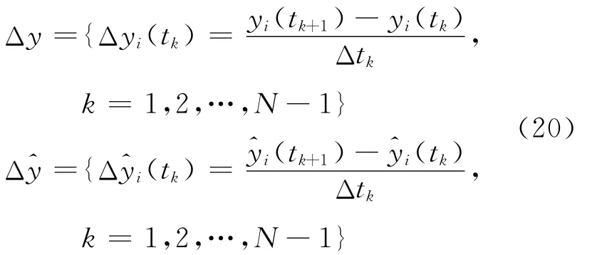
Step 2 Compute the absolute difference between the sequences and get the difference quotient sequences

Step 3 Compute the relation coefficient r（tk）and the AGCD GR（）

With the increase of p and m，the AGCD increases and gets more and more close to 1.That is，a more precise TVAR model can be established when p and mbecome larger.From the viewpoint of forecasting，however，it is not appropriate to choose arbitrarily large pand m.The mean squared error of the forecasts depends not only on the white noise variance of the fitted model，which will be smaller for a higher－order model，but also on errors，which will be larger for a higher－order model，arising from estimation of the model parameters.Furthermore，the increases of pand mmay yield false modes and over fitting，respectively，and result in large amount of computations.Hence，the optimal order pand dimension mshould be determined by choosing an appropriate value of AGCD，usually about 0.9for the identification of modal parameters based on ambient excitation test.

3.3 Determination of time－varying modal parameters

Consider the general case of a linear structure of nddegrees of freedom，modeled by FEM，as follows

where M，Kand Care the mass，stiffness，and damping matrices of dimension（nd×nd），respectively.q（t）and f（t）are the vectors of dimension（nd×1）for generalized displacement and external excitation，respectively.The parameter identification of Eq.（23）leads，by the application of the inverse Z－transform，to finding the parameters of a linear ARMA（2nd，2nd－1）model as follows［15］

with

For a time invariant structure，the coefficients ai（i＝1，2，…，2nd）and bi（i＝1，2，…，2nd－1）of the ARMA model are time－invariant.For a time－varying structure，however，these coefficients are time－varying.

Base on the equivalence relation of AMAR model and infinite－order AR model，the above ARMA（2nd，2nd－1）model can be replaced by an AR（∞）to avoid the nonlinear problem for solving the coefficients of MA model.In implementation，the coefficient estimation of an AR model of enough finite－orders can approximate the true coefficients of ARMA model.The coefficients of AR part contain the characteristics of frequencies and damping ratios of the system.As the AR model is an all－pole model，the transfer function at time instant tis

Thus，the instantaneous natural frequencies and modal damping ratios can be derived from the conjugate roots si（t），s（t）of the above transfer function as follows

4 Numerical Simulations

This section starts with the dynamic analysis of the beam model.The beam length，width and thickness are taken as 1，0.01and 0.01m，respectively.Furthermore，mass density，Young′s modulus，Poisson′s ratio and coefficient of thermal expansion of the beam material at the reference temperature are 2 700kg／m3，70GPa，0.3，and 2.3×10－5°C－1，respectively.Without loss of generality，the reference temperature is assumed to be 0°C in this paper.Fig.2and Fig.3show the variance of Young′s modulus［27］and coefficient of thermal expansion［28］versus temperature，respectively.

Fig.2 Variation of Young′s modulus vs.temperature

Fig.3 Variation of coefficient of thermal expansion vs.temperature

To discuss the advantage of the axially movable boundary for the simply－supported beam in Section 2，the ordinary axially immovable boundary must first and foremost be studied with a small change that makes ksequivalent to infinite in Eq.（1）.For simplicity，let beam A and beam B denote the simply－supported beams with two immovable boundaries and with an axially movable boundary，respectively.At the reference temperature，it is easy to obtain the first three natural frequencies of beam A，that is，23.1，92.4and 207.8Hz，respectively.One can readily get that the critical buckling temperature of beam A is only 3.57°C.Hence，beam A is easily to get buckled in a very low temperature.For this reason，attention in this paper is paid to beam B，where a spring with elastic constant 30kN／m is attached to the axially movable end of the beam.It is found that the critical buckling temperature of beam B rises to 455.7°C.Hence，all the numerical simulations hereinafter are made for beam B.

To study the time－varying modal parameters of beam B，the first three natural frequencies at the reference temperature should be determined.In case 1，the degeneration of material performance is taken into account.In case 2，only the effect of thermal stress is considered.In case 3，both effects of material performance degeneration and thermal stress are taken into consideration.

Fig.4shows how the first three natural frequencies of beam B change with the increase of temperature in three cases.It indicates that the natural frequencies of beam B decrease when temperature increases，where both the degeneration of material performance and the thermal stress inevitably matter.Their effects will be addressed in further discussion.

Fig.4 Variation of natural frequencies vs.temperature in three cases

Now，the dynamic response of beam B under a white noise excitation at the reference temperature can be computed by using the well－known Newmark－Beta algorithm.The parameters in the algorithm are set asγ＝0.5，β＝0.25andΔt＝0.001s.Then，the random decrement technique（RDT）is used to transfer the random response to free decays of the system.After the free decays are derived，the sparse time domain（STD）algorithm can be used to estimate the natural frequencies as shown in Table 1，where the modal parameters identified via RDT－STD method are compared with those identified via TVAR method.In Table 1，the first and the second natural frequencies identified via RDT－STD method and TVAR method are both close to their true values，and errors are within 0.5%of all.

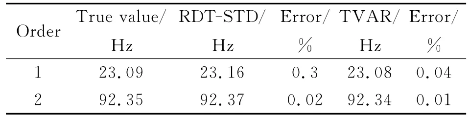
Table 1 Natural frequencies identified via RDT－STD and TVAR at reference temperature

Now，the study turns to the identification of time－varying natural frequencies of beam B subject to an unsteady heating.Fig.5illustrates three cases of unsteady temperature field of concern，i.e.，a linear increase，denoted as Temp 1；a linear increase followed by a constant，denoted as Temp 2；and a linear increase followed by a linear decrease，denoted as Temp 3.

Fig.5 Variation of temperature

To compute the dynamic response of the beam subjected to the above heating，it is necessary to interpolate the corresponding Young′s modulus and the thermal expansion coefficient of beam material according to the temperature at each time instant.Then，based on the axial equilibrium condition，it is straightforward to compute the axial thermal stress.After the material performance degradation and thermal stress are considered，the unit mass matrix，unit damping matrix，unit stiffness matrix and external force vector can all be determined.Finally，by integrating the unit matrixes into overall matrixes，the dynamic responses can be computed by using the Newmark－Beta algorithm.

To discuss the order selection for TVAR model，the case of Temp 1is taken as an example.The sampling number Nis very large and therefore the constant number Cof BIC criterion can be taken as 30.Fig.6shows the variation of BIC value versus the order pin the case of Temp 1.When pis assigned in the interval［12，40］，BIC values are small，but have fluctuations and reach several local minima.In this case，it is not possible to determine the minimal value.Hence，the order p can be preliminarily set within［12，40］，and then AGCD is used to determine the order p and dimension m simultaneously.Fig.7illustrates the variant of AGCD versus p and mindicating that AGCD increases and gets more and more close to 1with the increase of p and m.When dimension mis larger than 4，AGCD barely changes with the increase of mfor a constant order p.Here，pand mcan be taken as（28，4）or（27，6）respectively，and accordingly AGCD reaches a relatively large value，0.89.The real order of time－invariant AR model after the expansion of the time－varying parameters is p×（m＋1），and PNin Eq.（17）is a matrix of order p×（m＋1）.To decrease computation complexity，the order and dimension are taken as 28and 4，respectively.

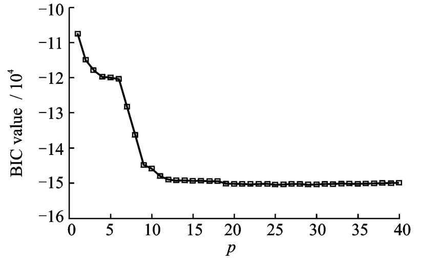
Fig.6 Variation of BIC

Fig.7 Variation of AGCD vs.dimension mand order p

For different cases of temperature variation，different order pand dimension mcan be determined simultaneously by combining BIC and AGCD.After selecting a suitable forgetting factor，the TVAR model can be established，and then the time－varying coefficients of TVAR model are derived via an RLS estimator.According to Eq.（27），the instantaneous natural frequencies can be obtained for the three cases of time－varying temperature.

In order to have a quantitative discussion，the mean absolute percentage error（MAPE）is defined as

where yiand＾yidenote the true value produced by the direct modal analysis and the identified value at the ith time instant respectively.Nis the total number of samplings.

Fig.8shows the instantaneous natural frequencies identified by the proposed method from the noise－free response of the TVAR model for three temperature variations.In Fig.8，the identified instantaneous frequency is capable of tracking temperature variation during the whole time duration.

Table 2gives the MAPE of natural frequencies in noise－free measurement，which shows that the identified instantaneous natural frequencies are close to their true values with high precision as the largest MAPE of them is smaller than 5%.

Fig.8 Instantaneous natural frequencies

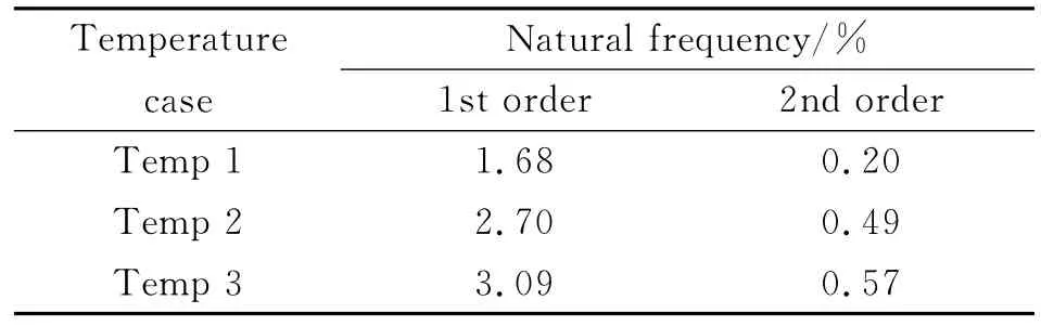
Table 2 MAPE for noise－free estimation

In practice，the measured data always contain corrupted noise of certain level.To demonstrate the robustness of the proposed method against the measurement noise，the simulated response data are assumed to be contaminated with a Gaussian noise of zero mean.More specifically，either 1%or 5%standard deviation of the noise－to－signal ratio（NSR）is used，and NSR is defined as

where sn is the standard deviation of the added noise and srs is the standard deviation of the response signal.In implementation，the numerical response is computed first and then the corresponding srs.Afterwards，snis determined from agiven NSR.A standard Gaussian white noise with a unit standard deviation is then generated，multiplied with the value sn，and then added to the response computed to produce the measured response.

The comparison of the MAPEs listed in Tables 2，3and 4shows that the processing of noisy responses reveals different observations of influence on natural frequencies.With an increase of NSR，all of MAPEs increase slightly for the natural frequencies identified in this paper.For example，MAPE of the first natural frequency in the case of Temp 1changes from 1.68to 1.70and 1.75for the cases of noise－free，NSR＝1%，and NSR＝5%，respectively.Meanwhile，the varia－tions of MAPEs of the identified natural frequencies and their true values are small.Based on the above discussion，one can safely draw an assertion that the measurement noise does affect the identification accuracy of natural frequencies slightly.

Table 3 MAPE for noisy estimation（NSR＝1%）

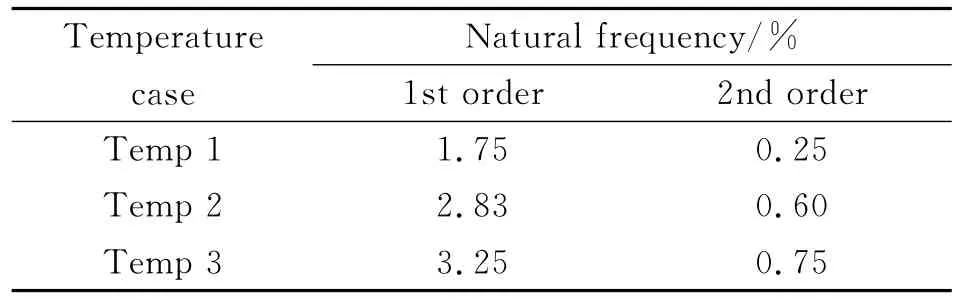
Table 4 MAPE for noisy estimation（NSR＝5%）

5 Conclusions

A systematic identification method is proposed for the time－varying modal parameters of a kind of thermo－elastic structure with sparse natural frequencies under unsteady heating conditions.The identification method is based on the TVAR model with time－varying coefficients for the structure to be identified from the input and output of the structure.These time－varying coefficients are expanded as a finite set of basis functions.The order of TVAR model and the dimension of basis functions are simultaneously determined via AGCD after a preliminary selection of order number from BIC.The identification method is applied to estimating the time－varying modal parameters of a simply－supported beam with an axially movable boundary subjected to different kinds of time－varying heating.The numerical simulations show that the identification method can estimate the instantaneous natural frequencies of the beam at each instant of heating process.The identified results are capable of tracking slow time－varying natural frequencies with high accuracy.The measurement noise usually causes slight shifts of identified frequencies.In future works，the method should be improved for identification of modal damping ratios with high accuracy，especially from noisy input and output data.

［1］ Fan X J.Thermal structures analysis and applications of high－speed vehicles［M］.Beijing：National Defence Industry Press，2009.（in Chinese）

［2］ McNamara J J，Friedmann P P.Aeroelastic and aerothermoelastic analysis in hypersonic flow：past，present，and future［J］.AIAA Journal，2011，49（6）：1089－1122.

［3］ Sun Y X，Fang D N，Soh A K.Thermoelastic damping in micro－beam resonators［J］.International Journal of Solids and Structures，2006，43：3213－3229.

［4］ Avsec J，Oblak M.Thermal vibrational analysis for simply－supported beam and clamped beam［J］.Journal of Sound and Vibration，2007，308：514－525.

［5］ Ghayesh M H.Coupled longitudinal－transverse dynamics of an axially accelerating beam［J］.Journal of Sound and Vibration，2012，331：5107－5124.

［6］ Yuan K H，Qiu Z P.Flutter analysis of composite panels in hypersonic flow with thermal effects［J］.Journal of Nanjing University of Aeronautics and Astronautics，2010，42（3）：313－317.（in Chinese）

［7］ Xiao S F，Chen B.Dynamic and buckling analysis of a thin elastic－plastic square plate in a uniform temperature field［J］.Acta Mechanica Sinica，2005，21：181－186.

［8］ Huang S Y，Wang Z Y.The structure modal analysis with thermal environment［J］.Missile and Space Vehicle，2009，5：50－52.（in Chinese）

［9］ Cohen L.Time－frequency distributions—A review［J］.Proceedings of the IEEE，1989，77（7）：941－981.

［10］Ibrahim G R，Albarbar A.Comparison between Wigner－Ville distribution－and empirical mode decomposition vibration－based techniques for helical gearbox monitoring［J］.Proceedings of the Institution of Mechanical Engineers，Part C：Journal of Mechanical Engineering Science，2011，225：1833－1846.

［11］Ghanem R，Romeo F.A wavelet－based approach for the identification of linear time－varying dynamical systems［J］.Journal of Sound and Vibration，2000，234（4）：555－576.

［12］Xu X，Shi Z Y，You Q.Identification of linear timevarying systems using a wavelet－based state－space method［J］.Mechanical Systems and Signal Processing，2012，26：91－103.

［13］Yu K P，Ye J Y，Zou J X，et al.Missile flutter experiment and data analysis using wavelet transform［J］.Journal of Sound and Vibration，2004，269（3－5）：899－912.

［14］Box G E，Jenkins G M，Reinsel G C.Time series analysis：forecasting and control［M］.Hoboken，NJ：John Wiley，2008.

［15］Yang S Z，Wu Y，Xuan J P，et al.Time series analysis in engineering application［M］.2nd Edition.Wuhan：Huazhong University of Science and Technology Press，2007.（in Chinese）

［16］Huang C S，Hung S L，Su W C，et al.Identification of time－variant modal parameters using time－varying autoregressive with exogenous input and low－order polynomial function［J］.Computer－Aided Civil and Infrastructure Engineering，2009，24（7）：470－491.

［17］Su W C，Liu C Y，Huang C S.Identification of instantaneous modal parameter of time－varying systems via a wavelet－based approach and its application［J］.Computer－Aided Civil and Infrastructure Engineering，2013，29（4）：279－298.

［18］Li Y，Wei H L，Billings S A.Identification of timevarying systems using multi－wavelet basis functions［J］.IEEE Transactions on Control Systems Technology，2011，19（3）：656－663.

［19］Poulimenos A G，Fassois S D.Output－only stochastic identification of a time－varying structure via functional series TARMA models［J］.Mechanical Systems and Signal Processing，2009，23：1180－1120.

［20］Poulimenos A G，Fassois S D.Parametric time－domain methods for non－stationary random vibration modelling and analysis—A critical survey and comparison［J］.Mechanical Systems and Signal Processing，2006，20：763－816.

［21］Akaike H.A new look at the statistical model identification［J］.IEEE Transactions on Automatic Control，1974，19（6）：716－723.

［22］Akaike H.A Bayesian analysis of the minimum AIC procedure［J］.Ann Inst Statist Math，1978，30（A）：9－14.

［23］Akaike H.A Bayesian extension of the minimum AIC procedure of autoregressive model fitting［J］.Biometrika，1979，66（2）：237－242.

［24］LüR.Rules of judging models for time series analysis［J］.Journal of National University of Defense Technology，1988，10（4）：97－106.（in Chinese）

［25］Guo L，Ljung L，Priouret P.Performance analysis of the forgetting factor RLS algorithm［J］.International Journal of Adaptive Control and Signal Processing，1993，7（6）：525－537.

［26］Lee S W，Lim J S，Baek S J，Sung K M.Time－varying signal frequency estimation by VFF Kalman filtering［J］.Signal Processing，1999，77：343－347.

［27］McLellan R B，Ishikawa T.The elastic properties of aluminum at high temperatures［J］.Journal of Physics and Chemistry of Solids，1987，48（7）：603－606.

［28］Nix F C，MacNair D.The thermal expansion of pure metals：copper，gold，aluminum，nickel，and iron［J］.Physical Review，1941，60：597－605.