HUANG Jing (黄静),

College of Civil Engineering, Tongji University, Shanghai 200090, China, E-mail: 1jhuang@tongji.edu.cn

PAN Cun-hong (潘存鸿)

Zhejiang Institute of Hydraulics and Estuary, Hangzhou 310020, China

KUANG Cui-ping (匡翠萍)

College of Civil Engineering, Tongji University, Shanghai 200090, China

ZENG Jian (曾剑), CHEN Gang (陈刚)

Zhejiang Institute of Hydraulics and Estuary, Hangzhou 310020, China

Experimental hydrodynamic study of the Qiantang River tidal bore*

HUANG Jing (黄静),

College of Civil Engineering, Tongji University, Shanghai 200090, China, E-mail: 1jhuang@tongji.edu.cn

PAN Cun-hong (潘存鸿)

Zhejiang Institute of Hydraulics and Estuary, Hangzhou 310020, China

KUANG Cui-ping (匡翠萍)

College of Civil Engineering, Tongji University, Shanghai 200090, China

ZENG Jian (曾剑), CHEN Gang (陈刚)

Zhejiang Institute of Hydraulics and Estuary, Hangzhou 310020, China

(Received April 8, 2013, Revised May 20, 2013)

To study the hydrodynamics of tidal bore, a physical modeling study is carried out in a rectangular flume with considerations of the tidal bore heights, the propagation speeds, the tidal current velocities, the front steepness, and the bore shapes. After the validation with the field observations, the experimental results are analyzed, and it is shown that: (1) the greater initial ebb velocity or the larger initial water depth impedes the tidal bore propagation, (2) the maximum bore height appears at an initial ebb velocity in the range of 0.5 m/s-1.5 m/s, (3) when the Froude number exceeds 1.2, an undular boreappears, after it exceeds 1.3, a breaking bore occurs, and after it exceeds 1.7, the bore is broken.

rectangular flume, initial flow condition, tidal bore height, bore shapes, propagation speed

Introduction

The tidal bore is a phenomenon happened in estuaries, where the tide forms a wave traveling up a river or a narrowing bay in the direction opposite to the river or bay’s current with a high velocity as a moving hydraulic jump. It occurs in at least 450 estuaries in the world, such as the Severn River in England, the Seine River in France, the Amazon River in Brazil and the Hooghly River in India[1], among which the tidal bore in the Qiantang River Estuary in China is the strongest.

The Qiantang River Estuary is a large tidal and funnel-shaped estuary. Through the Qiantang River Estuary an average discharge of about 952 m3/s[2]flows downstream, via the Hangzhou Bay into the East China Sea (see Fig.1). The Hangzhou Bay is about 100 km wide at its mouth (Luchaogang-Zhenhai cross-section), and it narrows to 20 km wide at the head of the bay, Ganpu cross-section, about 85 km away from the mouth with an increasing tidal range of up to 75%[3], the maximum tidal range of 9.0 m[3], and the flood tide accelerates as a result. At the upstream reach of Zhapu, there is a large sand bar of 130 km long and 10 m high above the river bottom along the channel axis[4], for which the water depth reduces sharply, and consequently the incoming tidal waves deform severely due to the enhanced shallow-water effect and finally the tidal bore develops, i.e., a sudden increase in the water level[4]. The geographic map of the Qiantang River Estuary is shown in Fig.1.

The tidal bore is an attracted research topic. Simpson et al.[5]measured the water level, the velocity, the Reynolds stress and the turbulent energy of the tidal bore in the Dee River Estuary, UK. Wolanskia et al.[6]studied the hydrodynamics of the undular tidalbore in the Daly River Estuary, Australia, with the field observations. Chanson[7,8]studied the turbulence beneath the undular bore, and performed the experiment in a rectangular horizontal channel to analyze the flow field, the effect of its mixing and diffusion of the undular bore. In China, Pan et al.[9]set up a 2-D numerical model with the well balanced Godunovtype scheme, and applied the model to study the tidal bore in the Qiantang River Estuary. They[10]also analyzed the characteristics of the tidal bore in the Qiantang River Estuary with the field data, and then built a 2-D mathematical model with the Kinetic Flux Vector Splitting (KFVS) scheme to successfully simulate the formation, the evolution and the dissipation of the Qiantang River tidal bore. Xie et al.[11]studied the hydrodynamic characteristics of the tidal bore in the Qiantang River Estuary with the field measurements. Yang et al.[12]generated tidal bores in the laboratory flume to measure the tidal bore heights, the propagation speeds and the tidal current velocities.

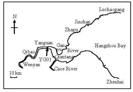
Fig.1 Geographic map of the Qiantang River Estuary

The flume experiment is widely applied in the studies of the tidal bore for it not only can simulate the various initial flow conditions but also can obtain exact measurements of the hydrodynamic data of the tidal bores and the bore fronts. However, most of the experimental studies were conducted in a still water before the tidal bore arrives, unlike in the real cases where the upstream water flows to the sea with a certain velocity. Furthermore, the existing experimental studies were seldom validated by the detailed field measurements.

In this study, the tidal bores with the different bore heights are generated in the glass rectangular flume under various initial flow conditions with respect to the water depths and the ebb velocities before the tidal bore arrives. In the experiments, the propagation speeds, the velocities, the heights, the shapes and the front steepness of the tidal bores are measured. The experimental results are validated by the field data measured at Yanguan reach in the Qiantang River Estuary in October, 2010[11]. The vertical distribution of the velocity and the correlations of the propagation speeds, the heights, the Froude number, the front steepness of the tidal bores are analyzed in the context of the hydrodynamics of the tidal bore for the designs and constructions of hydraulic structures in the Qiantang River Estuary.

1. Flume experimental model set-up

In this research, the measurements are made in a glass rectangular flume of 50 m in length, 1.2 m in width, 0.6 m in depth, and with zero bottom slope, equipped with the sluice gates at both ends, which can be raised and lowered. The transverters are installed to control the flows of the water pumps by changing their frequencies. By this means, it is possible to specify any desired initial conditions for the water depths and the ebb velocities. The ebb flows can be generated by lowering the sluice gate at the upstream end of the flume, whereas the tidal bores with a base flow can be generated by increasing the frequencies of the downstream transverter[13].

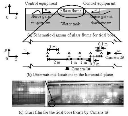
Fig.2 Layout of the gauge positions (“+” and “Δ” denote the locations of the observed bore heights and velocities respectively)

The tidal bore in the Qiantang River Estuary is formed by the rapid upstream narrowing, the shoaling, and the sharp deformation of the tidal wave[2]. The tidal bore is affected by the tide and the water depth before the tidal bore arrives. With the installation, the initial water depths and the ebb velocities before the tidal bore arrives and the tidal bore heights can be adjusted as the key parameters of the experiment with an undistorted model of the scale of 1 to 25 based on the gravity similarity criteria[14]. Totally 123 cases are considered in the flume experiment (see Table 1). Fig.2(a) is the schematic picture of the glass flume.

There are two video cameras mounted to measure the tidal bore front steepness (Camera 1#) with a glassfilm of 1.5 m long by 0.5 m high with 0.01 m uniform-space grids (see Fig.2(c)) and to capture the bore shapes (Camera 2#). 16 capacitive wave-height sensors are used to collect the tidal bore heights, and 6 Acoustic Doppler Velocimeters (ADV) at the different water depths of 0.125 m, 0.625 m,h /2,h,(H+ 2 h-0.25)/2and (H + h-0.25)(whereH andh denote the tidal bore height and the initial water depth, respectively) are installed to measure the velocities. The sampling interval is 0.01 s. The gauge positions are shown in Fig.2(b).

Table 1 Experimental parameters of initial water depths, initial ebb velocities and tidal bore heights with a model scale of 1 to 25

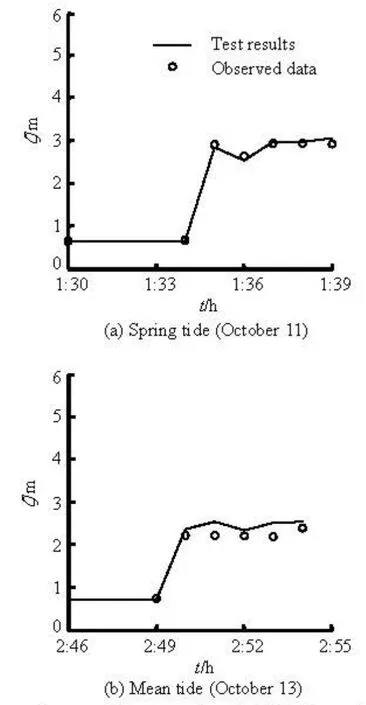
Fig.3 Comparisons of the experimental tidal bore heights with the prototype data in 2010 at YG01 station

2. Model validation

The prototype data collected in October 2010[11]at Yanguan reach, where the tidal bore is the strongest, are chosen to validate the model in this research.

Fig.4 Comparisons of the distributions of experimental velocities in the vertical direction with the field data in 2010 at YG01 station

The Percentage model Bias (PB), defined as Eq.(1), is adopted for the error analysis[15].

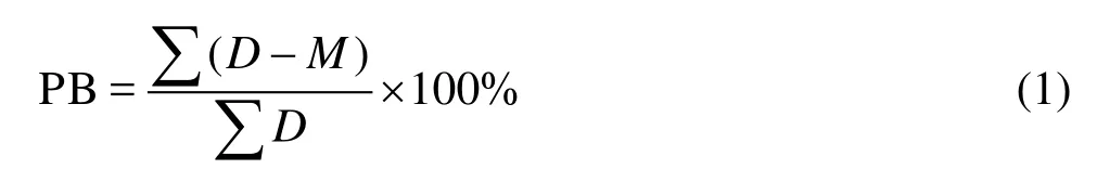
whereD represents the measured data, andMdenotes the corresponding test results. The results are considered as: excellent whenPB＜10%, very good when 10% ≤PB ＜20%, good when20% ≤PB≤40%and poor whenPB>40%[15].

The comparisons of the experimental results andthe field data measured at YG01 station (see Fig.1) in Yanguan reach[11]show that the tidal bore heights in the flume experiment agree well with the on-site observations (see Fig.3, whereζdenotes the water level) with the PB values of 0.14 % and 7.28 % for the two cases, and the distributions of the experimental velocities beneath the tidal bore fronts in the vertical direction are close to those at YG01 station (see Fig.4) with the PB values of 4.46 % and 3.38 % for the two cases. The good agreements show that the flume model can adequately reflect the characteristics of the actual tidal bore and be used to study the tidal bore in the Qiantang River Estuary.

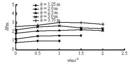
Fig.5 Relationship between H and vunder various initial water depths (the maximum initial ebb velocity under the initial water depth of 1.25 m is about 1.20 m/s, and that under the initial water depth of 2.0 m is 1.85 m/s)

3. Results and discussions

3.1 Tidal bore height

The tidal bore height is one of the indicators of the strength of the tidal bore, which increases with the increasing bore height. Figure 5 shows the relationship between H and vunder various initial water depths. It indicates that the maximum bore height appears at 0.5 m/s-1.5 m/s of the initial ebb velocity under various initial water depths (see Fig.5).

3.2 Propagation speed of the tidal bore

From the continuity and momentum equations, the propagation speed of the tidal bore can be expressed as[10]

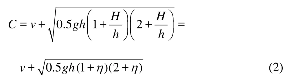
where C is the propagation speed of the tidal bore,h andvrepresent the initial water depth and the ebb velocity before the tidal bore arrives, respectively,H is the tidal bore height,η=H/ his the bore strength, andgis the gravity acceleration (see Fig.6). The calculated values of the bore propagation speeds agree well with those obtained in the flume experiment (see Fig.7(a)) with the relative error ranging from -10 % to 10 % (see Fig.7(b)).

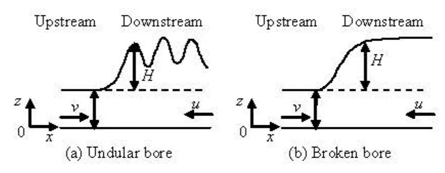
Fig.6 Definitions of the tidal bore

Fig.7 Comparison of the calculated Cand the experimental results

Our experimental results show that Cincreases linearly withHunder different initial water depths (see Fig.8) according to C=A1H +B1(where A1

and B1are listed in Table 2). And at the same ebb velocity before the tidal bore arrives, the bore propagation speed increases with the increase of the bore height, but the tidal bore with the same bore height decelerates when the initial ebbvelocity increases(seeFig.8).

Yanget al.[12]measured thetidal boreheights, the propagation speeds, and the tidal current velocities in the stationary initial water body in the concrete rectangular flume of 50 m long, 4 m wide and 1.2 m high, and came up with a relationship between the propa gation spe ed an d th e bore heig ht under the initial waterdepthof2.5m,expressedas C=1.448 H+4.874(R=0.98)(see Fig.9). Correspondingly, our experimentalresultcanbeexpressedasC= 1.319 H +5.116(R =0.98)(see Fig.9). It is evidentthat our result is similar to the result obtained by Yang et al.[12]when the initial flow is stationary.

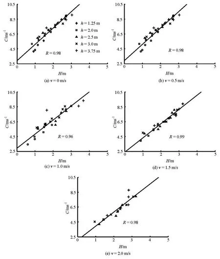
Fig.8 Relationship between C and Hunder various initial flow conditions (the maximum initial ebb velocity under the initial water depth of 1.25 m is about 1.20 m/s, and that under the initial water depth of 2.0 m is 1.85 m/s)

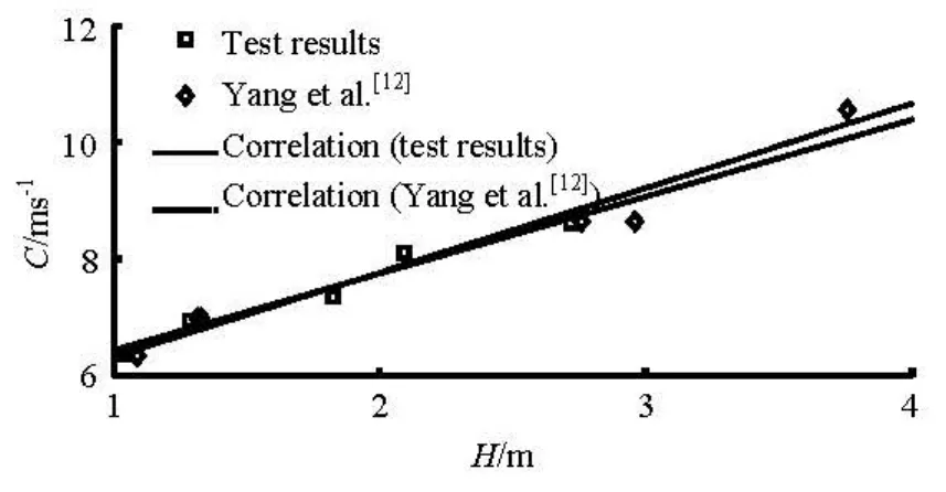
Fig.9 Comparison of our experimental result and the result by Yang et al.[12]under h =2.5 m when v=0 m/s

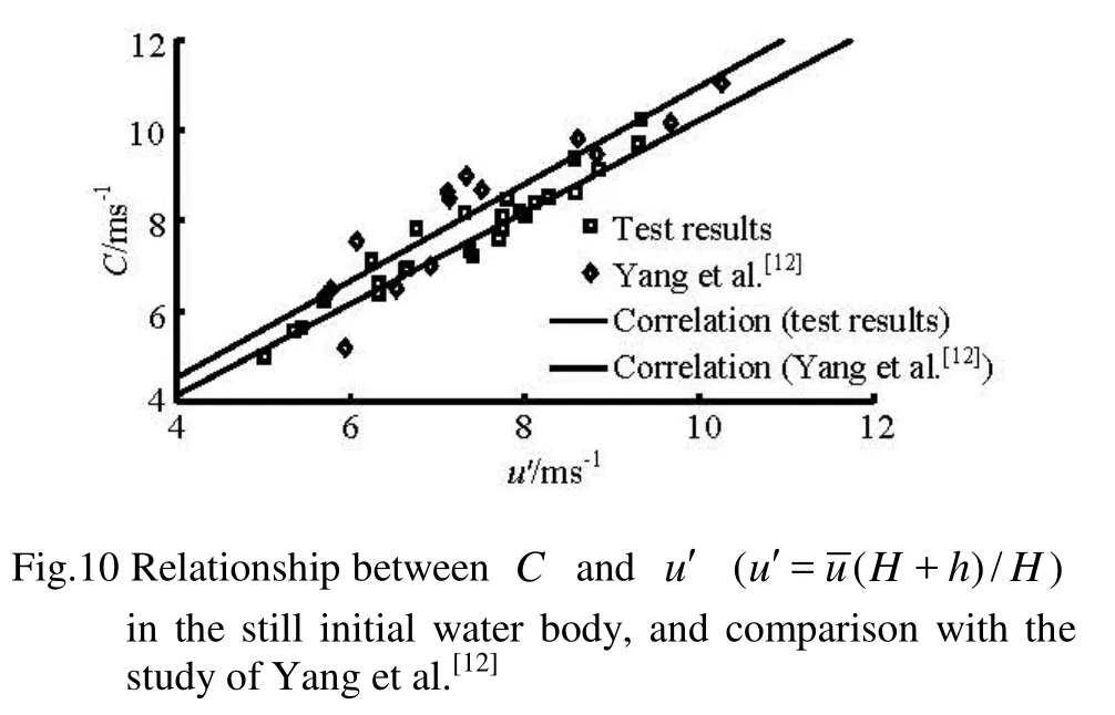
Fig.11 Relationship between C and u′′(u ′=( H + h)/H-vh/ H )

3.3 Distribution of the velocity beneath the tidal bore front in the vertical direction

On the arrival of the tidal bore, the flow in the research region is immediately controlled by the flood tide instead of the initial ebb flow (see Fig.4). The distribution of the velocity beneath the tidal bore front in the vertical direction assumes a parabolic curve. And the minimum velocity in the vertical direction occurs near the bottom due to the bottom resistance, whereas the maximum velocity of the undular bore with the bore height of about 1.1 m appears at the relative water depth of 0.3-0.8 and that of the brokenbore with the bore height larger than 1.8 m occurs at the relative water depth in the range of 0.5-0.8, and the distributions of the experimental velocities beneath the tidal bore fronts in the vertical direction under the initial water depth of 2.5 m with various initial ebb velocities are shown in Fig.12.

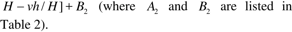
Table 2 Values of the constant coefficients in the formulas of C=A1H +B1and C= A2[( H +h)/H-vh/ H]+B2

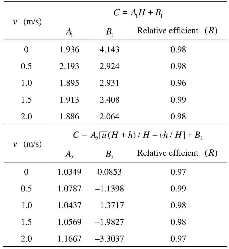
Table 2 Values of the constant coefficients in the formulas of C=A1H +B1and C= A2[( H +h)/H-vh/ H]+B2

v (m/s)11=+ C AH B 1A1BRelative efficient(R) 0 1.936 4.143 0.98 0.5 2.193 2.924 0.98 1.0 1.895 2.931 0.96 1.5 1.913 2.408 0.99 2.0 1.886 2.064 0.98 2 2 = [( + )//]+ C A u H h H vh H B -v (m/s) 2 A 2 BRelative efficient (R) 0 1.0349 0.0853 0.97 0.5 1.0787 –1.1398 0.99 1.0 1.0437 –1.3717 0.98 1.5 1.0569 –1.9827 0.98 2.0 1.1667 –3.3037 0.97

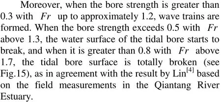
The velocity of the tidal bore with the same bore height decreases with the increase of the initial ebb velocity under the constant initial water depth, whereas when the initial ebb velocity is fixed, the velocity in the longitudinal direction decreases with the increase of the initial water depth before the tidal bore arrives (see Fig.13), due to the impediment of the upstream ebb flow to the flood tide.

3.4 Strength and Froude number of the tidal bore

The Froude number(Fr)of the tidal bore can be calculated by[1]

When v =0 m/s,Fr is linear withη, and their relationship can be expressed asFr=0.724η+1.305 (R =0.95)(see Fig.14). It is nearly the same as Fr= 0.744η+0.953(R=0.99)derived by Yang et al.[12](see Fig.14). Besides, under various initial flow conditions in this study, their relationships are also linear as Fr=0.884η+0.901(R =0.95)(see Fig.15).

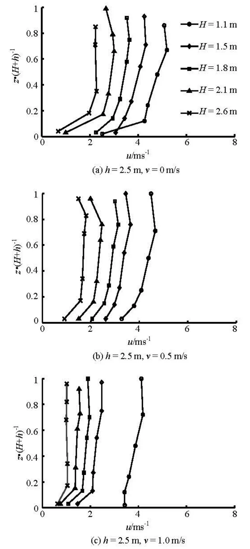
Fig.12 Distributions of experimental velocities beneath the tidal bore fronts in the vertical direction under h=2.5 m

3.5 Tidal bore shape

The tidal bore may assume various shapes during its propagation. When the tidal bore height is small, the undular bore appears with the series of the propelled waves (see Fig.16(a)) which is possibly caused bythe predominance of surface tension forces. But with a large bore height, the waves begin to break, and the breaking bore propagates in the channel (see Fig.16(b)). As soon as the tidal bore height is large enough, the bore is broken (see Fig.16(c)).

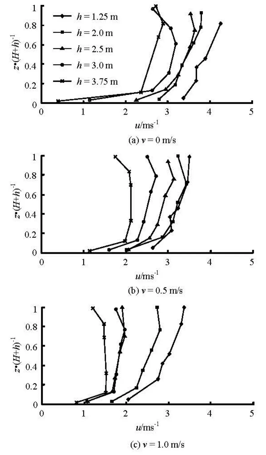
Fig.13 Distributions of experimental velocities beneath the tidal bore fronts with H =1.8 m in the vertical direction

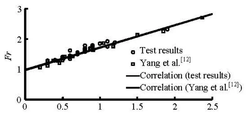
Fig.14 Relationship between Fr and η (η= H/ h)when v=0 m/s and the comparison with Yang et al.[12]

Fig.15 Relationship between Fr and ηunder various initial flow conditions

Fig.16 Shapes of the tidal bores and their fronts under h= 2.0 m when v=0.5 m/s (tidal bore shapes in the right figures and bore fronts in the left figures)

3.6 Steepness of the tidal bore frontAccording to the flat-bottom assumption, we have∂D/∂x= ∂ζ/∂x, Eq.(5) becomes

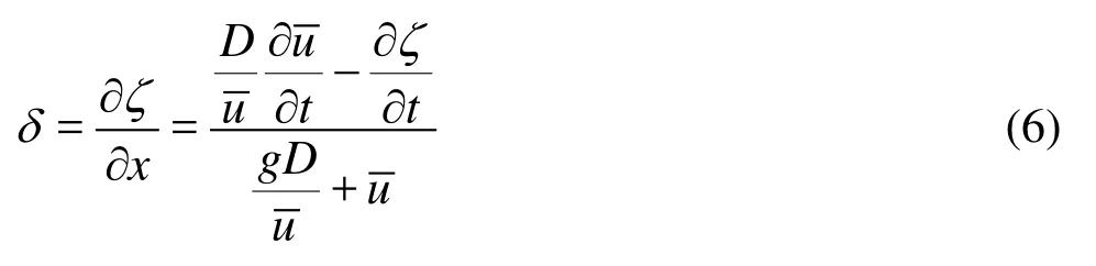
whereδrepresents the front steepness of the tidal bore,ζand Ddenote the water level and the total water depth respectively,uis the depth-averaged velocity in the longitudinal direction,t is the time, and

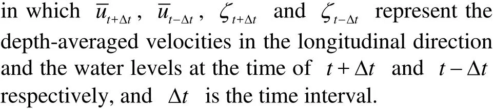
Table 3 Comparison of the experimental δand the calculatedδwith H =1.5 m

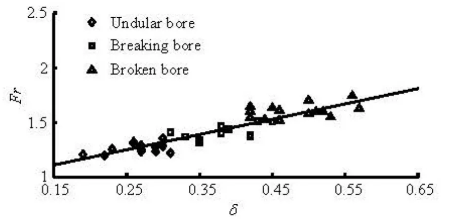
Fig.17 Correlation between Fr with δ

The comparison shows that the measured steepness of the tidal bore fronts is very close to the calculated results by Eq.(6) (see Table 3), with the relative error ranging from -3.57 % to 12.82 %, the averaged relative error of 4.96 %. And Frhas a positively linear relationship withδ, asFr=1.393δ+0.903 (R =0.91)(see Fig.17), whileδis also linear with ηas δ=0.415η+0.115(R=0.87)(see Fig.18). As soon as the front steepness exceeds 0.5, the water surface of the tidal bore is totally broken.

Fig.18 Correlation between δwithη

4. Conclusions

The tidal bores with the different bore heights are generated in the rectangular glass flume under various initial flow conditions with respect to the water depths and the ebb velocities before the tidal bore arrives. The propagation speeds, the velocities, and the bore heights of the tidal bores are measured, whilst the front steepness and the shapes of the tidal bores are captured. With the model scale of 1 to 25, the experimental results agree well with the field observed data at Yanguan reach in the Qiantang River Estuary.

The experimental results are analyzed, and the following conclusions can be reached.

(1) At the time of the tidal bore arrival, the flow in the research region is immediately controlled by the flood tide instead of the initial ebb flow. The minimum velocity in the vertical direction appears near the bottom for the large bottom resistance, while the maximum velocity mostly occurs in places from the middle layer to the surface layer.

The initial flow condition before the tidal bore arrives has a great impact on the tidal bore, i.e., the maximum bore height appears at the initial ebb velocity of 0.5 m/s-1.5 m/s, and the propagation of the tidal bore with the same bore height decelerates with the increase of the initial ebb velocity, the velocity of the tidal bore with the same bore height decreases with the increase of the initial ebb velocity in the constant initial water depth, whereas at a fixed initial ebb velocity, the velocity decreases with the increase of the initial water depth.

(2) The bore height,Fr, and the front steepness can all serve as the indicators for the tidal bore strength. The front slope of the tidal bore becomes steeper with the increasing bore strength, and the water surface is more broken with a largerFr . The tidal bore propagates faster with a larger bore height under the same initial ebb velocity.

(3) Tidal bore may assume various shapes during its propagation, i.e., the undular bore appears whenthe bore strength is greater than 0.3 withFr up to 1.2, the breaking bore occurs when the bore strength exceeds 0.5 with Frabove 1.3, and when the bore strength is greater than 0.8 withFrabove 1.7, the bore is broken.

Acknowledgement

We acknowledge the editor and three reviewers for their comments and suggestions to significantly improve the quality of the paper.

[1] CHANSON H. Tidal bores, aegire, eagre, mascaret, pororoca: Theory and observations[M]. Singapore: World Scientific, 2011, 37-92.

[2] PAN C., HUANG W. Numerical modeling of suspended sediment transport affected by tidal bore in Qiantang Estuary[J]. Journal of Coastal Research, 2010, 26(6): 1123-1132.

[3] PAN C., LIN B. and MAO X. Case study: Numerical modeling of the tidal bore on the Qiantang River, China[J]. Journal of Hydraulic Engineering, ASCE, 2007, 133(2): 130-138.

[4] LIN Bing-yao. Characteristics of the tidal bore in the Qiantang River[M]. Beijing, China: China Ocean Press, 2008, 40, 87, 170(in Chinese).

[5] SIMPSON J. H., FISHER N. R. and WILES P. Reynolds stress and TKE production in an estuary with a tidal bore[J]. Estuarine, Coastal and Shelf Science, 2004, 60(4): 619-627.

[6] WOLANSKI E., WILLIAMS D. and SPAGNOL S. et al. Undular tidal bore dynamics in the Daly Estuary, Northern Australia[J]. Estuarine, Coastal and Shelf Science, 2004, 60(4): 629-636.

[7] CHANSON H. Physical modelling of the flow field in all undular tidal bore[J]. Journal of Hydraulic Resea- rch, 2005, 43(3): 234-244.

[8] KOCH C., CHANSON H. Turbulent mixing beneath an undular tidal bore[J]. Journal of Coastal Research, 2008, 24(4): 999-1007.

[9] PAN Cun-hong, DAI Shi-qiang and CHEN Sen-mei. Numerical simulation for 2D shallow water equations by using Godunov-type scheme with unstructured mesh[J]. Journal of Hydrodynamics Ser. B, 2006, 18(4): 475-480.

[10] PAN Cun-hong, LU Hai-yan and ZENG Jian. Characteristic and numerical simulation of tidal bore in Qiantang River[J]. Hydro-Science and Engineering, 2008, (2): 1-9(in Chinese).

[11] XIE Dong-feng, PAN Cun-hong and LU Bo et al. Study on the hydrodynamic characteristics of the tidal bore on the Qiantang Estuary[J]. Chinese Journal of Hydro- dynamics, 2012, 27(5): 501-508(in Chinese).

[12] YANG Huo-qi, PAN Cun-hong and ZHOU Jian-jiong et al. Experiment study on hydraulic properties of tidal bore[J]. Water Resources and Power, 2008, 26(4): 136-138(in Chinese).

[13] HUANG Jing, LI Zui-sen and PAN Cun-hong et al. Application of Bore 2010 Control System to the flume experiment on the tidal bore[J]. Advances in Science and Technology of Water Resources Supplement, 2012, 32(S2): 28-30(in Chinese).

[14] HUANG Jing, PAN Cun-hong and CHEN Gang et al. Experimental simulation and validation of the tidal bore in the flume[J]. Hydro-Science and Engineering, 2013, (2): 1-8(in Chinese).

[15] ALLEN J. I., SOMERFIELD P. J. and GILBERT F. J. Quantifying uncertainty in high-resolution coupled hydrodynamic-ecosystem models[J]. Journal of Marine Systems, 2007, 64(3): 3-14.

10.1016/S1001-6058(11)60387-X

* Project supported by the National Natural Science Foundation of China (Grant No. 51109188), the National Key Basic Research Program of China (973 Program, Grant No. 2012CB957704) and the Ministry of Water Resources’ Special Funds for Scientific Research on Public Causes (Grant No. 201001072).

Biography: HUANG Jing (1985-), Female, Ph. D. Candidate

PAN Cun-hong, E-mail:panch@zjwater.gov.cn