FEI Zhengshun (费正顺), HU Bin (胡斌), YE Lubin (叶鲁彬) and LIANG Jun (梁军)**

State Key Lab of Industrial Control Technology, Institute of Industrial Control Technology, Zhejiang University,Hangzhou 310027, China

1 INTRODUCTION

Interest in dynamic optimization of chemical processes has increased significantly during the past years. Typical applications include control and scheduling of batch processes, transient and upset analysis,safety study and evaluation of control schemes. The model based dynamic optimization usually relies on the appropriate mathematical representation of the process.The mathematical models can be classified as white-box and data-driven models. White-box or mechanism models are constructed entirely from the first principles together with physical insight into the system behavior.Chemical processes are often modeled dynamically using differential algebraic equations (DAEs), with differential equations describing the dynamic behavior and algebraic equations denoting physical and thermodynamic relations [1]. However, the development of mechanism models based on detailed knowledge of physicochemical phenomena is usually quite difficult and time-consuming. In the manufacturing environment at present, the development of rigorous theoretical models may be impractical, or even infeasible.

Simplified data-based models from process operation data provide an attractive alternative way to mechanism modeling since less specific knowledge of the process is required. Studies on industrial process modeling suitable for the optimization based on process operation data without the knowledge of underlying mechanism are still at their infancy. The time-series model ARX (AutoRegressive with eXogenous inputs)is one of the common data-based models for capturing the dynamic behavior of the process [2]. An important issue in data-based modeling for a process is the collinearity of process variables, which is particularly serious when modeling data are collected in chemical processes with plenty of variables monitored in each process unit and many of them explain the same process event. One practical solution is to apply multivariate statistical projection based modeling technique of partial least squares (PLS), which takes into account the correlation of data [3]. The PLS approach can also reduce noise disturbances from collected process data.A number of investigations have addressed the data-based approach of PLS. Woldet al. [4] proposed a nonlinear PLS algorithm, which retains the framework of linear PLS but uses quadratic polynomial regression to fit the functional relation between each pair of latent variables. Qin and McAvoy [5] followed another way by incorporating neural networks into the inner mapping between input and output latent variables.Sharminet al. presented an application of PLS to build a soft-sensor to predict melt flow index using routinely measured process variables [6]. Baffiet al. developed a nonlinear dynamic PLS framework for application in model predictive control (MPC) [7] and Huet al. [8, 9]constructed multi-loop internal model control strategies based on the dynamic PLS framework.

The aim of this study is to provide a direct access for dynamic optimization using input and output data.The PLS method is used to model the process using historical operation data. For representing the dynamic and nonlinear behavior of the process, a structure of ARX cascaded with neural network (ARX-NN) is proposed to describe the inner relation between input and output latent variables. With the new ARX-NNPLS model, there is no need to solve DAEs iteratively for dynamic optimization.

In this study, a common dynamic optimization formulation is given and a new data-based modeling approach is proposed, in which the ARX-NN structure is used to relate the input and the output latent variables under the PLS framework. Using the developed ARX-NNPLS model, the dynamic optimization scheme is reconstructed and the algorithm for the optimization strategy is detailed. To demonstrate the effectiveness of the ARX-NNPLS model based dynamic optimization strategy, the polyethylene grade transition in gas phase fluidized-bed reactor is considered.

2 ARX-NNPLS MODEL BASED OPTIMIZATION STRATEGY

The mathematical expression for a dynamic optimization problem can be formulated as

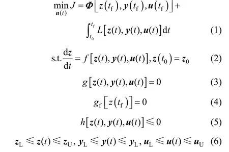
wherez(t) is differential state variables,y(t) is algebraic state variables,u(t) is control variables, andz0is initial values for differential state variables, andt0,tfare initial time and final time of the considered process.The process is modeled using differential algebraic Eqs. (2) and (3). Eq. (4) denotes the final point constraint and expression (5) is the inequality constraint.

To solve this kind of dynamic optimization problem, the control vector parameterization (CVP) approach [10, 11] is usually used, where control variables are discretized and the corresponding state variables are determined by solving DAEs. In the CVP approach the DAEs are solved in each optimization iteration. An outline for this method is shown in Fig. 1. A great deal of mechanism knowledge is needed to obtain the DAEs of the process, but the first principles are often difficult to know. Sometimes the model structure is known but the model parameters are unknown. In these cases, it is difficult to implement the process optimization.

Figure 1 The scheme of control vector parameterization approach

To provide an alternative way to achieve the optimization objective when less mechanism knowledge is known on the process, a PLS based dynamic nonlinear model is developed to model the dynamic process using the input and output data, in which the ARX-NN structure is used in the latent space to express the dynamic and nonlinear behavior of the process. Then the dynamic optimization operation can be implemented.

2.1 ARX-NNPLS modeling

Partial least squares (PLS) [2, 12], also known as projection to latent structures, is a latent variable based method used for the linear modeling of the relationship between a set of predictor variables and a set of response variables. From a practical view, PLS is a technique that can decompose a multivariate regression problem into a series of univariate regression problems.

Before PLS modeling, the process data needed for modeling should be properly scaled. The data-based model will be developed with the following assumptions:(1) the process is controlled using a computer with piecewise constant manipulated inputs; (2) measured output trajectories are obtained in the form of data vectors sampled at regular and sufficiently small time intervals; and (3) the historical database for developing the data-based models is sufficiently large. Here,the control variables are used as input and the output consists of differential and algebraic state variables.Two blocks of data samples are collected and properly scaled to start the PLS modeling procedure. LetX(sizen×l) represents the input data set andY(sizen×s)represents the output data set. PLS technique always requires two steps to accomplish the model.

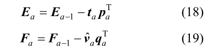
The first step is to use the NIPALS (nonlinear iterative partial least square) iterative algorithm [12] to break matricesXandYinto a certain number of bilinear terms,

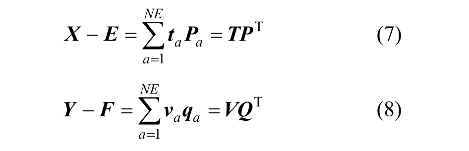
wheretaandvaare latent score vectors,paandqaare corresponding loading vectors,NEis the number of latent variables,TandVdenote score matrices,PandQrepresent loading matrices forXandYblocks, andEandFare residual matrices ofXandY, respectively.

The second step is to acquire the PLS inner model.The PLS inner model reveals the algebraic relationship between input and output latent variables,

wherebais the coefficient determined by least squares method.

To extend the PLS approach to represent the dynamic and nonlinear characteristics, an ARX time series model cascaded with neutral network structure in the PLS inner relation is developed to obtain arbitrary nonlinear dynamic description for the process. The overall diagram of the model structure is shown in Fig. 2,whereP+denotes the appropriate inverse of the input loading matrixP. The structure is employed to fit the relation between the input latent matrixTand the output latent matrixV.

For theath PLS latent space, the mathematical formulation of the ARX structure is

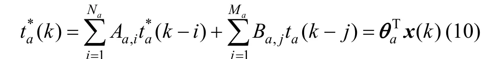
where(k) is the output of the ARX model, which will be served as the input for the next segment of neural network,NaandMaare the time lags for outpuTt and input variables of ARX. The parameter setsθaandx(k) are defined as

The nonlinearity between output latent variables and transformed input latent variables is represented using neural network as follows (assuming that only one hidden layer is used in the neural network).

whereF(·) denotes the implicit nonlinear relation of a neural network unit,W1,aandW2,aare the weights in the hidden layer,β1,aandβ2,adenote the bias in the hidden layer, andσ(·) is the centered sigmoid function used in the work of Qin and McAvoy [5]. As each single in single out (SISO) ARX-neural network model in the PLS subspace can be designed and trained without interfering with others, the PLS framework will greatly reduce the computation time to train the neural networks for multivariable processes.

A neural network with one hidden layer is sufficient in most function approximation problems [13]. In this work, a two-layer network with one centered sigmoidal function hidden layer and one linear function output layer is implemented to represent the nonlinear characteristics in the latent space. The number of hidden units and latent variables are determined by a simplified cross-validation method [5].

As a result, the following inferential model ofYbased the neural network outputva(k) can be written as

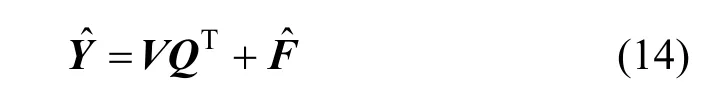
where ˆYis the inferential output and ˆFis the residual matrix in the final PLS model. Using the ARX-NNPLS model, for arbitrary input variable matrixX, the inferential output ˆYcan be obtained.

The modeling algorithm based on the ARX-NN structure is as follows.

Step 1 Scale input and output matricesXandYto have zero mean and unit variance. Set0=EX,0=FYand 1a=.

Step 2 Call the NIPALS algorithm to extract score vectorstaandva.

Step 3 Using the ARX-NN structure to build the inner model.

Step 4 Determine the loading vectors ofXandY.

Step 5 Calculate the residuals after extracting theath factor.

Step 6 Seta=a+1 and return to Step 2 until allNEprinciple factors (latent variables) are calculated.Then there is no useful information in residual matricesENEandFNE. The number of latent variablesNEis determined by cross-validation [5].

2.2 Dynamic optimization using ARX-NNPLS models

The conventional CVP approach depends on the DAEs model of the process, while with the proposed ARX-NNPLS modeling approach, it is possible to employ the model directly into the CVP based optimization scheme.

In the ARX-NNPLS model, the control variables are used as the input, while the differential and algebraic state variables are served as output. The input control vector is constructed asu= [u1u2⋅⋅⋅ul], wherelis the number of input variables. The output vector is constructed asy= [y1y2⋅⋅⋅ys], wheresis the total number of differential state variables and algebraic state variables. It is assumed thatKsample points are collected in the time horizon [t0,tf] of the dynamic process. With the ARX-NNPLS model developed, for any input vectoru(k) at sample pointk, the corresponding output vectory(k) is deduced as

Therefore, the dynamic process can be modeled by the ARX-NNPLS approach, and the DAEs in the dynamic optimization problem [Eqs. (1)-(6)] can be substituted by the ARX-NNPLS model when the mechanism model is unavailable. Because the differential and algebraic variables are all treated as output variables,the objective function can be reformulated as

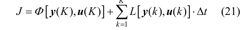
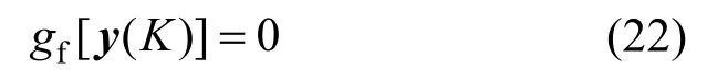
where Δtis the sampling time interval. BecauseKpoints are sampled in the process, the final values of state variables are those at theKth sample point. The final point constraint can be expressed as

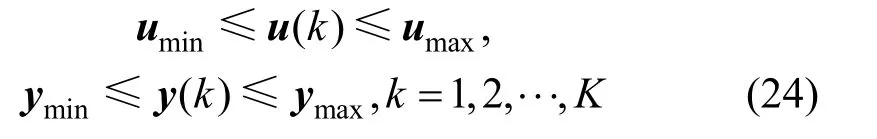
It is difficult to deal with the inequality constraint in the form of expression (5). Since the input and output trajectories are discretized and implemented as piecewise constant trajectory, it is sufficient to satisfy the constraint condition at each sampling point. The inequality constraint can be formulated as

Similarly, the upper and lower bounds on input and output trajectories can also be changed into the constraint at sampling instants.

Hence, the original dynamic optimization problem is reconstructed as

The aim of the optimization is to choose suitable decision variablesU= [u( 1 )⋅ ⋅⋅u(k) ⋅ ⋅⋅u(K)]Tto minimize the objective function. The decision variableUof the new optimization problem, Eq. (25), is the input for the ARX-NNPLS model shown in Eq. (20). Note that the deduced optimization problem is a normal nonlinear programming (NLP) problem, so any standard NLP algorithm [1] (SQP, genetic algorithms, inter point algorithm,etc.) can be used.

A schematic diagram of the ARX-NNPLS based dynamic optimization algorithm is showed in Fig. 3.The output matrixYcan be obtained from the ARXNNPLS model when input matrixUis given. The objective function is calculated fromYand the input matrixU. A new set of decision variableUis chosen in the NLP solver and the process is repeated until the optimum is achieved.

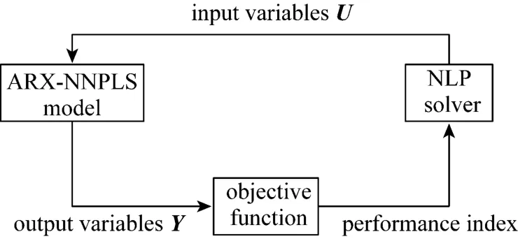
Figure 3 The scheme of ARX-NNPLS based approach

The steps of the ARX-NNPLS based dynamic optimization approach are as follows. A flowchart for this approach is given in Fig. 4.

Figure 4 A flowchart of ARX-NNPLS dynamic optimization approach

Step 1 Set the input matrixUto the initial valueU0.

Step 2 With the input and output loading matricesPandQdetermined in the ARX-NNPLS modeling procedure, compute input scoresTbyUandP,T=UP+.

Step 3 PassTto the ARX m*odeling part to calculate the dynamic model out*putT.

Step 4 Use the outputTas the input for the neural network to obtain the nonlinear outputV.

Step 5 Compute the overall outputTYbased the output scoresVof neural networkY=VQ

Step 6 Calculate the performance index throughUandY.

Step 7 Calculate the newUin NLP solver.

Step 8 Check whether two criterionsare satisfied: if yes, go to Step 9, otherwise go to Step 2, whereε1andε2are small tolerance values.

Step 9 Achieve the optimal valueUopt=U.

Step 10 Calculate the final optimal outputYoptat the optimal inputUoptusing the ARX-NNPLS model in a similar way.

Compared to the conventional CVP optimization strategy based on DAEs, neither parameterization nor iterative solving of DAEs is needed in this dynamic optimization structure, as the ARX-NNPLS model gives a proper representation for the dynamic behavior of the process. In other words, ARX-NNPLS modeling uses the discretization treatment for the original dynamic optimization problem, which is converted into a normal nonlinear programming problem. The MATLAB optimization toolbox can be used to solve the NLP problem, where a serial of input sampling points in the dynamic time domain is chosen as the decision variable.

3 APPLICATION IN POLYETHYLENE GRADE TRANSITION PROCESS

3.1 Process description

Here we consider a gas-phase fluidized-bed reactor process as it is a widely used industrial process for ethylene polymerization [14-16]. A simplified gas-phase fluidized-bed reactor is showed in Fig. 5.The gas stream comprised of ethylene, hydrogen, butene and nitrogen is fed at the bottom of the reactor and catalyst particles are continuously fed into the reactor to produce polymer particles. Recycle gases are pumped into the bottom of the reactor after mixing with the fresh gas stream. A heat exchanger is used to remove the polymerization heat from the recycle stream. To remove excessive inert components and impurities, a fraction of recycle gas is vented at the top of the reactor. The polymer product is removed from the bottom of the reactor periodically.

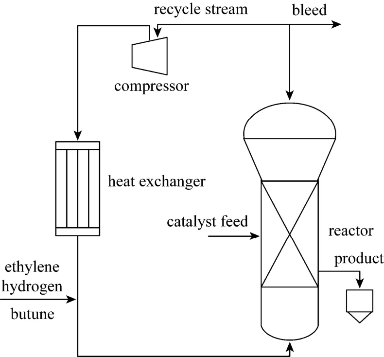
Figure 5 Diagram of polyethylene fluidized-bed reactor

Polyethylene has wide applications in industrial products and everyday life. To satisfy diverse market demands, polyolefin companies often produce different grades of polymer products in the same reactor by changing the operating conditions [15]. Melt index (the amount of melted polymer that can be squeezed through a standard orifice in 10 min) and density are often used for the specification of polyolefin products.

3.2 ARX-NNPLS model for ethylene polymerization

In an ethylene polymerization reaction, the final product quality index of cumulative melt indexMIcand cumulative densityDcare determined by reactor temperatureT, molar ratio of hydrogen to ethylene in the cycle gas ([H2]/[M1]), and molar ratio of comonomer to ethylene in the cycle gas ([M2]/[M1]). To build the ARX-NNPLS model, reactor temperature is assumed to be uniform in the transition process, and the two ratios [H2]/[M1] and [M2]/[M1] serve as input variables whileMIcandDcserve as output variables for the process. Process data are selected with a sampling interval of 10 min for modeling (while the practical operation data can be collected in a higher frequency).The data from 600 samples are available to build the dynamic nonlinear PLS model, while test data with 600 samples are generated in a similar way. Fig. 6 shows the polymer specifications,MIcandDc, used as the training data. It is important that the data to be used for training cover the possible variation in the domain of the problem. Each neural network is trained separately in PLS latent space without interfering with others. Since the network will go to the nearest local minimum from the initial point as the training proceeds, the best linear model between latent variables is used to initialize the hidden unit in order to find a better minimum with high computational efficiency.

To regress the relationship between input latent variables and output latent variables, the ARX-NN structure is established, and a complete list of model parameters is demonstrated in Table 1. The modeling result using ARX-NNPLS is showed in Fig. 7.

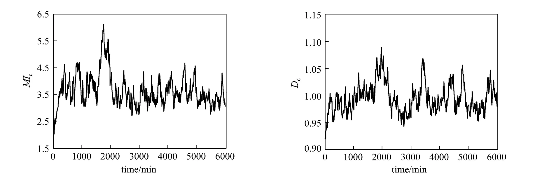
Figure 6 Time series plot for MIc and Dc

Table 1 ARX-NN model parameters in grade transition process

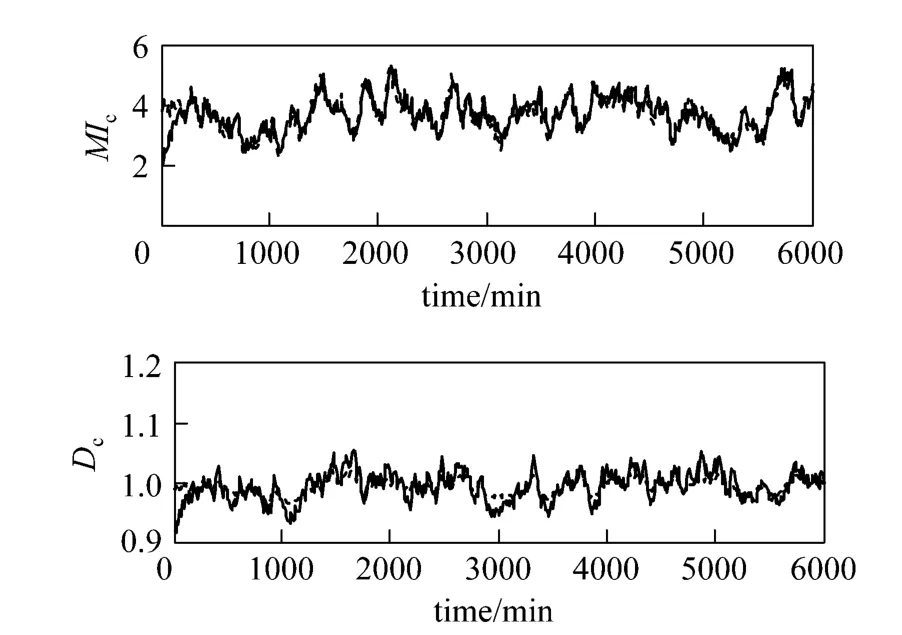
Figure 7 Comparison of prediction from ARX-NNPLS model with experiment (solid line: actual values; dashed line:predicted values)

3.3 Grade transition optimization based ARXNNPLS model

A considerable amount of off-specification polymer is usually produced during grade transitions. It is important to minimize the amount of off-spec polymer in an optimization problem [17-21], so that the optimal operation variables and quality variables can be determined. Here two polyethylene grades are considered in the transition operation, as stated in Table 2.

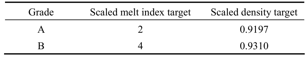
Table 2 Two grades considered in transition study

In order to minimize the off-specification polymer in the grade transition operation, a widely used objective function penalizing the deviations from targets is used [17, 20, 21].

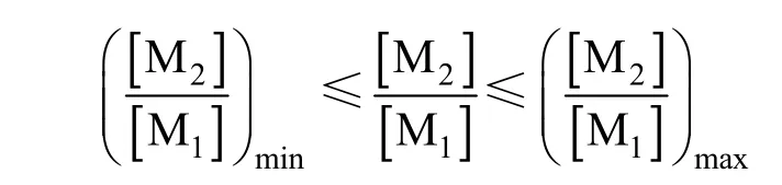
whereMIfandDfare target values of melt index and density, respectively,ω1andω2denote weighting factors. When the objective function is minimum, the amount of off-specification polymer produced is the least. Based on the ARX-NNPLS model developed,the optimization problem is depicted as

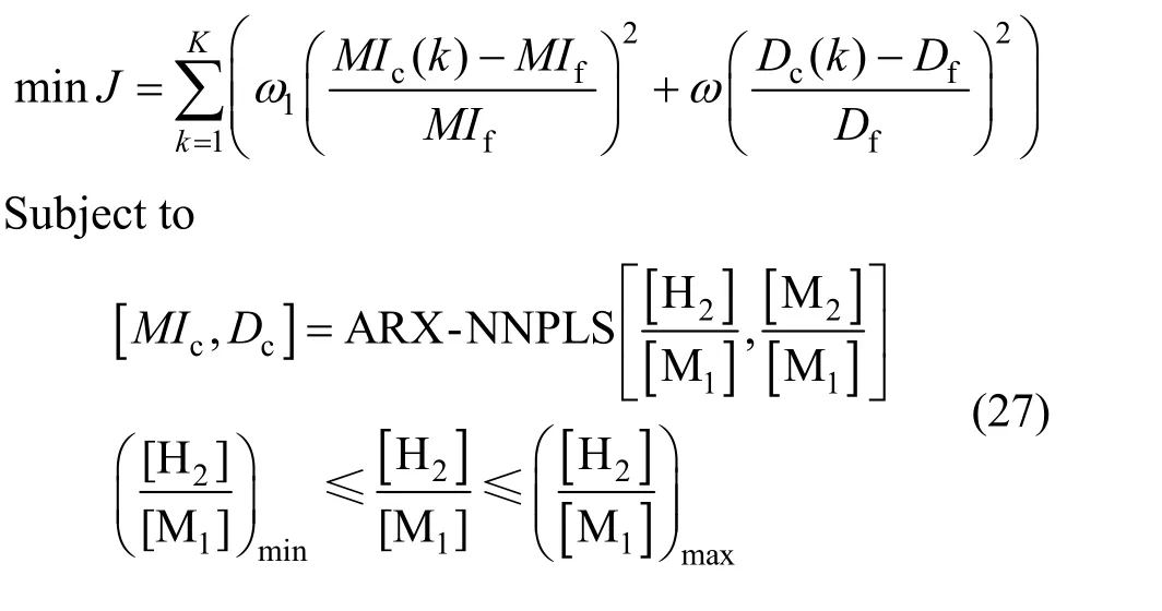
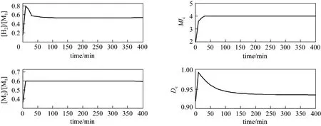
Figure 8 Optimal profiles for input and output variables (grade A→grade B)

The grade transition optimization problem is virtually a function optimization problem, the aim of which is to achieve the optimal input operating profiles. While the developed ARX-NNPLS model is used in the optimization scheme, the original function optimization problem is translated into a finite-dimensional optimization problem and common NLP algorithm can be used to solve it directly. For the transition process from grade A to grade B, the weighting factorsω1andω2are all set to 1 and the grade transition optimization problem is solved using the MATLAB optimization toolbox. Then the optimal profiles for the input and output variables can be determined, as shown in Fig. 8.It indicates that the quality indexMIcandDcof polyethylene products will gradually grow to the target values after the transition process, and the least amount of off-specification polymer is produced at the same time when the performance index is minimized.

In order to confirm that the ARX-NNPLS model can be used in general grade transition optimization problems, a simplified first-principle model for ethylene polymerization proposed by McAuley and Mac-Gregor [14] is used for comparison. For the gas-phase fluidized-bed ethylene polymerization process, DAE model equations are whereMIiandDidenote instantaneous melt index and density,τis the polymer-phase residence time in the reactor,ki(i= 1 ,2,⋅ ⋅ ⋅,5 ) andpj(j= 1 ,⋅⋅⋅,4 ) are parameters to be determined.

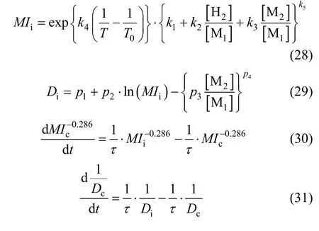
The result from the ARX-NNPLS model based optimization is compared to that from the conventional dynamic optimization. The original optimization problem is constructed by substituting the developed ARXNNPLS model with the differential algebraic Eqs.(28)-(31). The mechanism model based optimization problem is solved by the conventional CVP method.The computing notebook platform comprises a T7250(2.0 GHz) processor and 2 GB memory. The CPU time elapse with ARX-NNPLS model based approach is about 28.13 s, which is greatly less than that with the CVP method (about 186.10 s). The final optimal quality profiles determined by the two methods are illustrated in Fig. 9. The quality index grows quickly to the target value using the present data-based model,especially for melt indexMIc. In other words, the transition time for the operation with the present method is less than that with the CVP method.

As shown in Fig. 8, a quite large overshoot appears in the trajectory of the quality indexDc, which may not be permitted in practical operation. For reducing the overshoot and controlling the cumulative densityDcrigorously in an allowable region, additional constraint condition can be added to the optimization problem. Here the transient process constraintDc(t)＜0.98 is added to Eq. (27) and the developed ARX-NNPLS model is used. It is sufficient to ensure the constraint at each sampling point and the added constraint is

Figure 9 Comparison of optimal profiles from ARX-NNPLS based method with CVP result (dashed: CVP; solid:the present method)

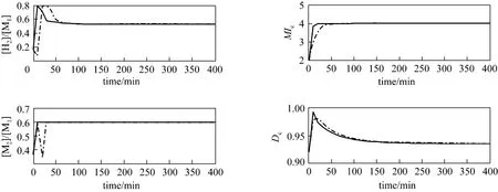
Figure 10 Optimal profiles for constraint case using ARX-NNPLS model based strategy (dashed: with constraint; solid: without constraint)

Solving this optimization problem with quality index constraints, the optimal profiles are shown in Fig. 10,which is compared to the results withoutDcconstraints, Eq. (27). The quality indexDcis restricted in the allowable domain, but it takes longer time for all the input and output variables to approach the steady-state values.

4 CONCLUSIONS

In order to provide a practical access of dynamic optimization to the case where the DAEs of the process is difficult to obtain, an ARX-NNPLS model based dynamic optimization strategy is proposed, in which a data-based modeling approach using ARX cascade with neural network under the PLS scheme is developed. The ARX-NNPLS model can be used directly in the control vector parameterization based optimization scheme and a normal nonlinear programming problem will be achieved, which can be solved by any standard NLP algorithm.

The approach is applied in optimization of polyethylene grade transition process. Using the input and output data of the process, a data-based ARX-NNPLS model is built and the optimal grade transition operation profiles are determined. Compared to the results of trajectory optimization based on a simplified first-principle model, optimal trajectories of quality index obtained with the present method move faster to target values while the computing time is much less. The overshoot in optimal profiles of quality index can be reduced by adding some inequality constraints in the optimization.

1 Biegler, L.T., Grossmann, I.E., “Retrospective on optimization”,Comput.Chem.Eng., 28 (8), 1169-1192 (2004).

2 Qin, S.J., “Recursive PLS algorithms for adaptive data modeling”,ComputChem Eng, 22 (4-5), 503-514 (1998).

3 Wold, S., Ruhe, A., Wold, H., Dunn, W.J., “The collinearity problem in linear-regression—The partial least-squares (PLS) approach to generalized inverses”,Siam Journal on Scientific and Statistical Computing, 5 (3), 735-743 (1984).

4 Wold, S., Kettanehwold, N., Skagerberg, B., “Nonlinear PLS modeling”,Chemometrics and Intelligent Laboratory Systems, 7 (1-2),53-65 (1989).

5 Qin, S.J., McAvoy, T.J., “Nonlinear PLS modeling using neural networks”,Comput Chem Eng, 16 (4), 379-391 (1992).

6 Sharmin, R., Sundararaj, U., Shah, S., Griend, L.V., Sun, Y.J., “Inferential sensors for estimation of polymer quality parameters: Industrial application of a PLS-based soft sensor for a LDPE plant”,Chem.Eng.Sci., 61 (19), 6372-6384 (2006).

7 Baffi, G., Morris, J., Martin, E., “Non-linear model based predictive control through dynamic non-linear partial least squares”,Chem Eng Res Des, 80 (A1), 75-86 (2002).

8 Hu, B., Zheng, P.Y., Liang, J., “Multi-loop internal model controller design based on a dynamic PLS framework”,Chin.J.Chem.Eng.,18 (2), 277-285 (2010).

9 Hu, B., Zhao, Z., Liang, J., “Multi-loop nonlinear internal model controller design under nonlinear dynamic PLS framework using ARX-neural network model”,Journal of Process Control, 22 (1),207-217 (2012).

10 Vassiliadis, V.S., Sargent, R.W.H., Pantelides, C.C., “Solution of a class of multistage dynamic optimization problems (1) Problems without path constraints”,Ind.Eng.Chem.Res., 33 (9), 2111-2122(1994).

11 Wang, Y., Seki, H., Ohyama, S., Akamatsu, K., Ogawa, M., Ohshima,M., “Optimal grade transition control for polymerization reactors”,Comput.Chem.Eng., 24 (2-7), 1555-1561 (2000).

12 Geladi, P., Kowalski, B.R., “Partial least-squares regression—A tutorial”,Anal.Chim.Acta, 185, 1-17 (1986).

13 Basheer, I.A., Hajmeer, M., “Artificial neural networks: Fundamentals, computing, design, and application”,J.Microbiol.Meth., 43 (1),3-31 (2000).

14 McAuley, K.B., MacGregor, J.F., “Online inference of polymer properties in an industrial polyethylene reactor”,AIChE J, 37 (6),825-835 (1991).

15 Bonvin, D., Bodizs, L., Srinivasan, B., “Optimal grade transition for polyethylene reactorsviaNCO tracking”,Chem.Eng.Res.Des., 83(A6), 692-697 (2005).

16 Mostoufi, N., Kiashemshaki, A., Sotudeh-Gharebagh, R., “Two-phase modeling of a gas phase polyethylene fluidized bed reactor”,Chemical Engineering Science, 61 (12), 3997-4006 (2006).

17 Padhiyar, N., Bhartiya, S., Gudi, R.D., “Optimal grade transition in polymerization reactors: A comparative case study”,Ind.Eng.Chem.Res., 45 (10), 3583-3592 (2006).

18 McAuley, K.B., MacGregor, J.F., “Optimal grade transitions in a gas-phase polyethylene reactor”,AIChE J, 38 (10), 1564-1576 (1992).

19 Wang, J.D., Yang, Y.R., “Study on optimal strategy of grade transition in industrial fluidized bed gas-phase polyethylene production process”,Chin.J.Chem.Eng., 11 (1), 1-8 (2003).

20 Chatzidoukas, C., Perkins, J.D., Pistikopoulos, E.N., Kiparissides, C.,“Optimal grade transition and selection of closed-loop controllers in a gas-phase olefin polymerization fluidized bed reactor”,Chemical Engineering Science, 58 (16), 3643-3658 (2003).

21 Flores-Tlacuahuac, A., Biegler, L.T., Saldivar-Guerra, E., “Optimal grade transitions in the high-impact polystyrene polymerization process”,Ind.Eng.Chem.Res., 45 (18), 6175-6189 (2006).