Huaqing Liu(刘华清), Rui Jiang(姜锐),†, Junfang Tian(田钧方), and Kaixuan Zhu(朱凯旋)

1Key Laboratory of Transport Industry of Big Data Application Technologies for Comprehensive Transport,Ministry of Transport,Beijing Jiaotong University,Beijing 100044,China

2College of Management and Economics,Tianjin University,Tianjin 300072,China

3Suzhou Institute of Technology,Jiangsu University of Science and Technology,Zhangjiagang 215600,China

Keywords: traffic flow,connected and automated vehicles(CAVs),lane drop,optimization-based control algorithm,Heuristic rules-based algorithm

1. Introduction

The deployment of connected and automated vehicles(CAVs) is regarded as an effective method to improve traffic performance.[1–3]On the one hand, CAVs are expected to shorten time gap and smooth traffic oscillations, so that traffic capacity increases[4]and energy consumption reduces.[5]On the other hand, the passing sequence of CAVs from different lanes in conflicting areas can also be determined and optimized to maximize the utilization of spaces.[6]

Merging of traffic flow can be treated as a usual conflicting scenario.[7–12]One approach to deal with merging traffic flow is heuristic rules-based algorithm (HRA).[13–15]One common method in this approach is to introduce the virtual vehicles. For example, in Unoet al.,[16]in order to make smooth merging, a virtual vehicle is generated by mapping a vehicle on one lane onto another lane. Simulation results showed the feasibility of the merging control algorithm. Lu and Hedrick[17]and Luet al.[18]proposed the concept of virtual platoon, which effectively avoids a two-point boundary value problem. Based on the concept, a rather general adaptive algorithm is provided, which has been implemented and tested with automated cars.In a recent work,[19]we introduced restriction of the command acceleration caused by the virtual leading vehicle, which significantly improves the passenger’s comfort level.

The other approach for the longitudinal control of CAVs at merges is optimization-based control algorithm.[20–23]Several optimization-based control algorithms have been formulated and the trajectories of CAVs can be solved.[24]The trajectories usually should satisfy several constraints, including speed constraint, acceleration constraint, jerk constraint, and safety constraint. A widely used optimization-based control(OCA)is proposed in Refs.[25,26],which maximizes average travel velocity of each vehicle. Nevertheless,a comprehensive study on the performance of this optimization-based control algorithm as well as the comparison with the HRA is lacking.

Motivated by the fact, this paper investigates phase transition in traffic flow of CAVs under the OCA proposed in Refs.[25,26]at lane drop on two-lane highway and compares the performance between the OCA and the HRA proposed in Ref. [19]. It is found that (i) capacity under the HRA (denoted asCH)is smaller than capacity under the OCA;(ii)the travel delay is always smaller under the OCA, but driving is always much more comfortable under the HRA;(iii)when the inflow rate is smaller thanCH,the HRA outperforms the OCA with respect to the fuel consumption and the monetary cost;(iv) when the inflow rate is larger thanCH, the HRA initially performs better with respect to the fuel consumption and the monetary cost,but the OCA would become better after certain time. Our study is expected to help for better understanding of the two different types of algorithm.

The rest of the paper is organized as follows.In Section 2,the two control algorithms are reviewed. Section 3 compares the performances of the two control algorithms. Section 4 gives the conclusion.

2. Review of two control algorithms

2.1. Geometric layout

Figure 1 shows the geometric layout of a lane drop on a two-lane highway.As reported in Ref.[19],we assume that inflow rate is the same on the two lanes and all vehicles on lane 2 change lane only at the lane drop,i.e., the merging point is at the lane drop. Note that different from that in Ref.[19],the end of the control zone is downstream of the lane drop. Otherwise,under the OCA,large jerk would occur when vehicles exit the control zone.

Fig.1. The geometric layout of a lane drop on a two-lane highway.

2.2. Longitudinal control algorithm outside control zone

As reported in Ref. [19], we assume that constant time gap control algorithm is used outside control zone in which the command acceleration and the actual acceleration are

wheregis the actual spacing andgdesireis the desired spacing

Moreover,the physical constraints below should be satisfied:i

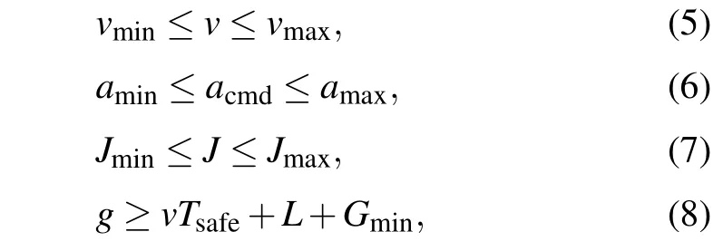
n whichJ=da/dtis the jerk of vehicle. Other notations and parameters are listed in Table 1.

When vehicles enter control zone,the merging sequence is determined by ’first-in-first-out’ (FIFO) principle. If two vehicles enter at the same time instant,vehicle on lane 1 is regarded as the’first-in’one. Note that since the vehicles move in the FIFO principle,we calculate the vehicle trajectory in a sequence order. Therefore,once the constraints(7)and(8)are not satisfied,we re-calculate the vehicle trajectory and let the vehicle decelerate earlier.

Table 1. Notations and parameters.

2.3. Control algorithms in control zone

2.3.1. Heuristic rules-based algorithm

We briefly review the HRA proposed in Ref.[19]. In the control zone, a virtual set of vehicles is constructed, which includes all vehicles in the control zone. We number these vehicles based on the arriving order at the control zone. If two vehicles arrive at the control zone at the same time, vehicle from lane 1 is numbered before that from lane 2. In the virtual set,if the preceding vehicle of the ego one is not on the same lane, then we map the preceding vehicle onto the ego lane,which becomes a virtual leading vehicle of the ego one.

The command accelerationacmd,egoof ego vehicle concerning vehicle on the same lane is calculated as

The command accelerationacmd,virtualconcerning virtual leading vehicle is calculated as

whereacmd,limis the restriction onacmd,virtualto improve driving comfort level.

The command acceleration, used as the input to lower control,is determined as

Inside the control zone, the physical constraints (5)–(8)should also be satisfied.Note that the longitudinal–lateral couplings (9)–(11) are applied symmetrically for the vehicles on both lanes.

2.3.2. Optimization-based control algorithm

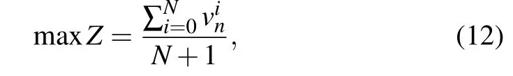
In the OCA proposed in Refs. [25,26], the trajectory of each vehicle is obtained by maximizing the average speed in control zone. The objective function and constraints are formulated as

subject to

Herenmeans vehicle number. The algorithm is based on the length of discrete time step ΔT, andidenotes the time step.Nmeans the total number of time steps that vehiclenneeds to move across the control zone. The values of parameters in the two algorithms are listed in Table 2, see also Ref. [19].The control gain parameterska,kv, andkgshould guarantee that traffic flow is stable,and other parameters are in the usual ranges reported in the literature.

Table 2. The values of parameters.

3. Evaluation and comparison of the control algorithms

The length of the studied road section is set to 8000 m and the control zone is from 5000 m to 7000 m. The lane drop is at 6900 m. The inflows are stochastic. A vehicle enters withvmax=30 m/s and the probabilityp0if the last vehicle on the lane is beyondL+Gmin+Tgvmax. By generating vehicles in this way,the headways of vehicles follow shifted negative exponential distribution, as observed in real traffic. When the leading vehicle reaches the exit atx=8000 m, it is removed and the second vehicle becomes the new leading one and its acceleration is assumed to be unchanged.

3.1. Capacity

Figure 2(a)shows the dependence of the inflow and outflow rate on entering probabilityp0under the two control algorithms. In the simulation,20 runs were carried out for each entering probabilityp0. The results are averaged over the 20 runs. One can see that there exists a threshold of entering probability under each control algorithm. The thresholdp0=p0,c,HRA≈0.072 under HRA andp0=p0,c,OCA≈0.075 under OCA. Whenp0is below the threshold, the outflow equals to the inflow and traffic flow is free. Whenp0exceeds the threshold,congestion forms and the outflow is equal to the capacity, which is 2562 vehicles/h under the HRA and 2612 vehicles/h under the OCA. Thus, OCA performs better than HRA in terms of capacity. This is related to the different movement of vehicles in the vicinity of the lane drop. As shown in Fig.2(b),under OCA,vehicles decelerate for merging at the lane drop and accelerates quickly downstream of the lane drop;under the HRA,vehicles accelerate smoothly in the vicinity of the lane drop. The quick acceleration downstream of the lane drop yields larger throughput than smooth acceleration.

Fig.2. (a)The dependence of the inflow and outflow rate on the entering probability p0. (b)Typical speed profiles of vehicles in the vicinity of the lane drop. The entering probability p0=0.09.

3.2. Spatiotemporal pattern

To understand evolution of the traffic flow of CAVs under the two algorithms,the spatiotemporal patterns are presented.Figure 3 shows the results in a typical low-level inflow situation atp0=0.06.One can see that under the OCA,remarkable decelerations are observed upstream of the lane drop. Downstream of the lane drop, the decelerating vehicles quickly accelerate, see Figs. 3(a) and 3(c). Under the HRA, the decelerations are mainly observed when vehicles enter the control zone. Then they accelerate smoothly in the control zone, see Figs.3(b)and 3(d). Accordingly,notable jerks are mainly observed near the lane drop under the OCA(Fig.3(e))and near the entrance of control zone under the HRA(Fig.3(f)).

Fig.3. The spatiotemporal patterns under(top)OCA and(bottom)HRA at p0=0.06. (a),(b)Speed(unit: m/s);(c),(d)notable acceleration/decelerations with|a|＞0.5(unit: m/s2);(e),(f)notable jerk with|J|＞0.5(unit: m/s3).

Figure 4 shows the results in a typical medium-level inflow rate atp0=0.074. Under the OCA,due to the stochastic inflow, although the mean inflow rate is smaller than the capacity, sometimes the inflow rate could exceed the capacity.Once the inflow exceeds the capacity,congestion occurs at the entrance of control zone. The congestion will gradually dissipate when the inflow rate falls below the capacity. As a result,notable acceleration/decelerations and jerks are observed near both the lane drop and the entrance of control zone, see Figs.4(c)and 4(e).

Under the HRA, the inflow exceeds the capacity and congestion will occur. Nevertheless, the congestion initially emerges in the control zone rather than at the entrance of control zone,as indicated by the arrow.Then the congestion propagates upstream. When the downstream front of the congestion arrives at the control zone entrance,it will be fixed there.The upstream front of congestion further propagates upstream and the congestion region gradually expands. As a result,notable acceleration/decelerations and jerks initially emerge in the control zone and near the control zone entrance. With the propagation of congestion,they will be observed near the control zone entrance and/or the upstream front of congestion,see Figs.4(d)and 4(f).

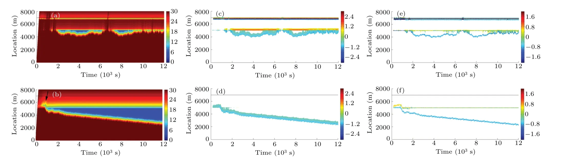
Fig.4.The spatiotemporal patterns under(top)OCA and(bottom)HRA at p0=0.074.(a),(b)Speed(in units:m/s);(c),(d)notable acceleration/decelerations with|a|＞0.5(in units: m/s2);(e),(f)notable jerk with|J|＞0.5(in units: m/s3).

Figure 5 shows the results in a typical high-level inflow rate atp0=0.09. Under the OCA,congestion emerges at the control zone entrance. Then the upstream front of the congestion propagates upstream and congestion region expands. As a result, notable acceleration/decelerations and jerks are observed near the lane drop, the entrance of control zone, and the upstream front of congestion,see Figs.5(c)and 5(e).

Under the HRA, the emergence of congestion (as indicated by the arrow) and its propagation is similar to that in the medium-level inflow rate situation. Notable acceleration/decelerations and jerks are also similar,see Figs.5(d)and 5(f). Since the capacity is smaller than that under the OCA,the propagation speed of upstream front of congestion under the HRA is larger than that under the OCA.

Fig.5.The spatiotemporal patterns under(top)OCA and(bottom)HRA at p0=0.09.(a),(b)Speed(in units:m/s);(c),(d)notable acceleration/decelerations with|a|＞0.5(in units: m/s2);(e),(f)notable jerk with|J|＞0.5(in units: m/s3).

3.3. Travel delay

Figure 6 compares the performance of HRA and OCA with respect to travel delay at three typical levels of inflow rate: (i) low level,p0=0.06＜p0,c,HRA; (ii) medium level,p0,c,HRA＜p0=0.074＜p0,c,OCA;(iii)high level,p0=0.09＞p0,c,OCA. One can see that no matter what level of the inflow rate, the travel delay under OCA is always smaller than that under HRA.Here travel delay is defined as the difference between the actual travel time and the free travel time.

In the low-level inflow situation, the difference is small,which is less than 1 s on average,see Fig.6(a).In the mediumlevel and the high-level situations, the difference increases with the vehicle number. The latter a vehicle enters,the larger the difference is,see Figs.6(b)and 6(c).This is because under the HRA,the capacity is smaller so that congestion propagates faster. In contrast, under the OCA, either there is no congestion(in the medium-level inflow situation)or congestion propagates slower(in the high-level inflow situation).

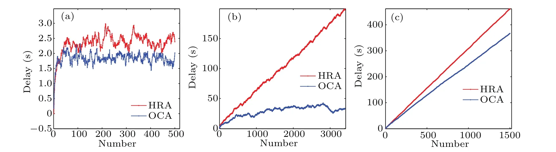
Fig.6. Travel delay at(a) p0=0.06;(b) p0=0.074;(c) p0=0.09.

Next we compare the travel delay in the control zone,in the road sections upstream and downstream of the control zone,respectively. Figure 7 shows the results in the low-level inflow situation. The travel delay upstream of the control zone is neglectable under both algorithms, see Fig. 7(a). In the control zone, as expected, the travel delay under the OCA is smaller because the OCA aims to maximize the vehicle speed,see Fig.7(b). In contrast,downstream of the control zone,the travel delay under the OCA is larger,see Fig.7(c). This is because, under the OCA,some vehicles decelerate significantly when approaching the lane drop.Thus,on average,the vehicle speed downstream of the control zone is smaller,see Figs.3(a)and 3(b). Note that the difference of delay is around+1.3 s in the control zone,and is around–0.8-s downstream of the control zone. Therefore,in total,the travel delay is smaller under the OCA.

Figures 8 and 9 show the results in the medium-level and high-level inflow situation, respectively. The results in the control zone and downstream of the control zone are the same as in the low-level situation,i.e., the travel delay under the OCA is smaller in the control zone but larger downstream of the control zone. However, upstream of the control zone,travel delay is initially roughly equal between the HRA and the OCA(Fig.8(a))or smaller under the HRA(Fig.9(a)). But it gradually increases because congestion occurs. In contrast,under the OCA,either there is no congestion and travel delay fluctuates around 10 s–20 s(Fig.8(a))or the congestion is not as strong as that under the HRA and travel delay grows slower(Fig.9(a)). Thus,after some time,travel delay becomes larger under the HRA.

Fig.7. Travel delay(a)upstream of the control zone,(b)in the control zone,and(c)downstream of the control zone. The inflow is in low level(p0=0.06).

Fig.8. Travel delay(a)upstream of the control zone,(b)in the control zone,and(c)downstream of the control zone. The inflow is in medium level(p0=0.074). In panel(a),the delay under the HRA exceeds that under the OCA at vehicle number i ≈480,which enters at t ≈1311 s.

Fig.9. Travel delay(a)upstream of the control zone, (b)in the control zone, and (c) downstream of the control zone. The inflow is in high level(p0=0.09). In panel(a),the delay under the HRA exceeds that under the OCA at vehicle number i ≈430,which enters at t ≈1074 s.

3.4. Fuel consumption

To measure the fuel consumption of vehicles,we use the following model as in Ref.[27]

in whichKijis constant coefficients listed in Table 3 fora ≥0 anda ＜0.

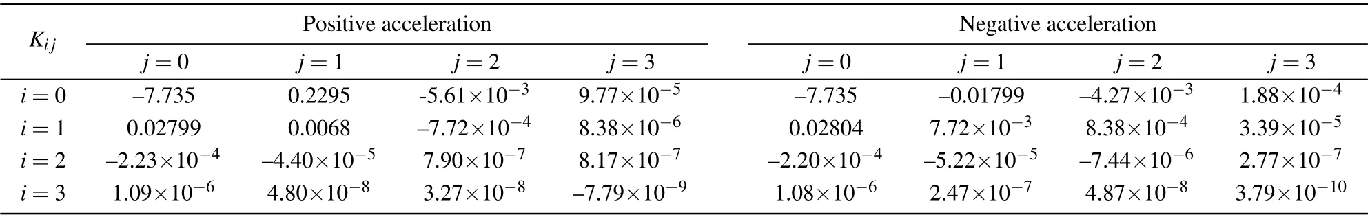
Table 3. Coefficients of fuel consumption for a ≥0 and a ＜0.

Figure 10 compares the performance of HRA and OCA in terms of fuel consumption at the three typical levels of inflow rate. In the low-level inflow situation, fuel consumption under the HRA is always smaller than that under the OCA,see Fig.10(a). In the medium-level and high-level inflow situation, fuel consumption is initially smaller under the HRA,see Figs.10(b)and 10(c). However,under the OCA,fuel consumption either does not grow(in medium-level inflow situation) or grows slower (in high-level inflow situation). Therefore,fuel consumption under the HRA will exceed that under the OCA after certain time. Nevertheless, the time is rather long, which is about five hours in both the medium-level and the high-level inflow situations. The time duration is even larger than the duration of usual rush hours, which is about 2～3 hours. Therefore, from the perspective of real application, the HRA outperforms the OCA with respect to the fuel consumption.

We also compare fuel consumption in the three road sections. Figure 11 shows the results in the low-level inflow situation. Since the vehicles move with maximum speed,the fuel consumption upstream of the control zone is almost the same under the two algorithms,see Fig.11(a). However,in the control zone and downstream of the control zone, fuel consumption is larger under the OCA,see Figs.11(b)and 11(c). This is because the acceleration/deceleration behavior under the OCA is not as smooth as that under the HRA,cf. Figs.3(a)–3(d).

Fig.10. Fuel consumption at(a) p0=0.06;(b) p0=0.074;(c) p0=0.09.

Fig.11. Fuel consumption(a)upstream of the control zone,(b)in the control zone,and(c)downstream of the control zone. The inflow is in low level(p0=0.06).

Fig.12. Fuel consumption(a)upstream of the control zone,(b)in the control zone,and(c)downstream of the control zone. The inflow is in medium level(p0=0.074). In panel(a),the fuel consumption under the HRA exceeds that under the OCA at vehicle number i ≈1185,which enters at t ≈3233 s.

Figures 12 and 13 show the results in the medium-level and high-level inflow situations,respectively. As in low-level inflow situation, fuel consumption is larger under the OCA in the control zone and downstream of the control zone, see Figs. 12(b),12(c)and 13(b),13(c). However,as shown in Figs.12(a)and 13(a),upstream of the control zone,after some transient time,the fuel consumption under the HRA would increase with the vehicle number due to the formation of congestion. In contrast,under the OCA,the fuel consumption either does not increase with vehicle number(in the medium-level inflow situation)or increases slower(in the high-level inflow situation). While the difference of fuel consumption becomes larger and larger upstream of the control zone, the difference does not change in the control zone and downstream of the control zone. Therefore, after enough long time,the total fuel consumption will become larger under the HRA.

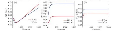
Fig.13. Fuel consumption(a)upstream of the control zone,(b)in the control zone,and(c)downstream of the control zone. The inflow is in high level(p0=0.09). In panel(a),the fuel consumption under the HRA exceeds that under the OCA at vehicle number i ≈430,which enters at t ≈1074 s.

3.5. Monetary cost

Whereas the OCA yields smaller travel delay,sometimes it yields larger fuel consumption than the HRA. Thus, we make an integrated evaluation of the two costs by converting travel time cost and fuel consumption cost into monetary cost.

According to NUMBEO (Numbeo is the world’s largest cost of living database, see www.numbeo.com (accessed on 2022 March 2)),in China,the mean salary is 6825.46¥/month,and the price of gasoline is 7.32¥/L(¥denotes Chinese Yuan and 1¥≈0.1572 US$). Therefore,the unit cost of travel time is 42.66 ¥/h (The unit cost is calculated based on that each month has 20 workdays and each workday has eight work hours).In USA,the mean salary is 3602$/month and the price of gasoline is 0.73$/L.Therefore,the unit cost of travel time is 22.51$/h.

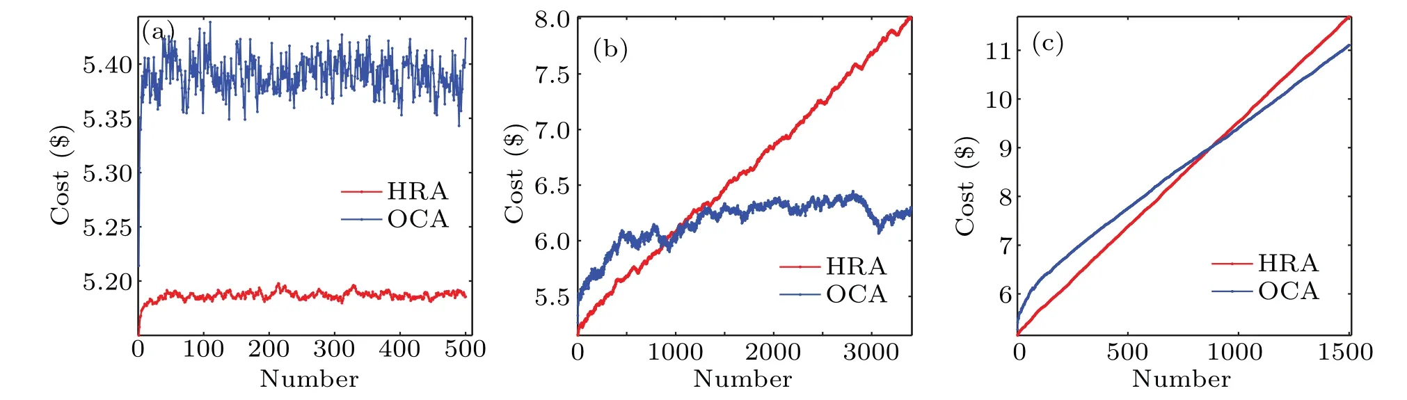
Fig.14. Monetary cost in China at(a) p0=0.06;(b) p0=0.074;(c) p0=0.09. In panel(b),the monetary cost under the HRA exceeds that under the OCA at vehicle number i ≈1000,which enters at t ≈2730 s. In panel(c),the monetary cost under the HRA exceeds that under the OCA at vehicle number i ≈880,which enters at t ≈2200 s.

Fig.15. Monetary cost in USA at(a) p0=0.06;(b) p0=0.074;(c) p0=0.09. In panel(b),the monetary cost under the HRA exceeds that under the OCA at vehicle number i ≈180,which enters at t ≈491 s. In panel(c),the monetary cost under the HRA exceeds that under the OCA at vehicle number i ≈250,which enters at t ≈623 s.

Figure 14 shows the monetary cost in China at the three typical levels of inflow rate. In the low-level inflow situation,monetary cost is smaller under the HRA,see Fig.14(a). In the medium-level and high-level inflow situations,initially monetary cost is also smaller under the HRA.However,after about 2730 s (2200 s), the monetary cost under the HRA exceeds that under the OCA in the medium-level (high-level) inflow situation,see Figs.14(b)and 14(c). Considering that the rush hour duration is about 2–3 hours,practically it might be better to use the HRA firstly, and then switch to the OCA after certain time. Finally,after the rush hour,switch back to the HRA again. In the future work, the switching strategy needs to be further investigated.

Figures 15 shows the monetary cost in USA at the three typical levels of inflow rate. The results are similar to that in China. However, in the medium-level and high-level inflow situations,the monetary cost under the HRA exceeds that under the OCA much earlier than in China. Therefore, practically the switch from HRA to OCA should be made much earlier.

3.6. Comfort level

In the literature,J2is used to measure the instantaneous comfort level and the cumulativeJ2of each vehicle denotes the comfort level when driving through overall road section,seee.g., Refs. [19,23]. We denote the cumulativeJ2as ˆJ2,thus

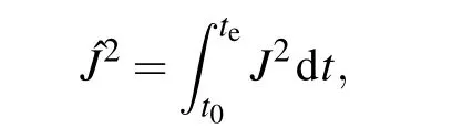
in whicht0andteare the entering and leaving time of ego vehicle,respectively. A larger ˆJ2means a lower comfort level.

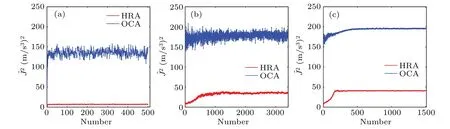
Fig.16. Comfort level at(a) p0=0.06;(b) p0=0.074;(c) p0=0.09.

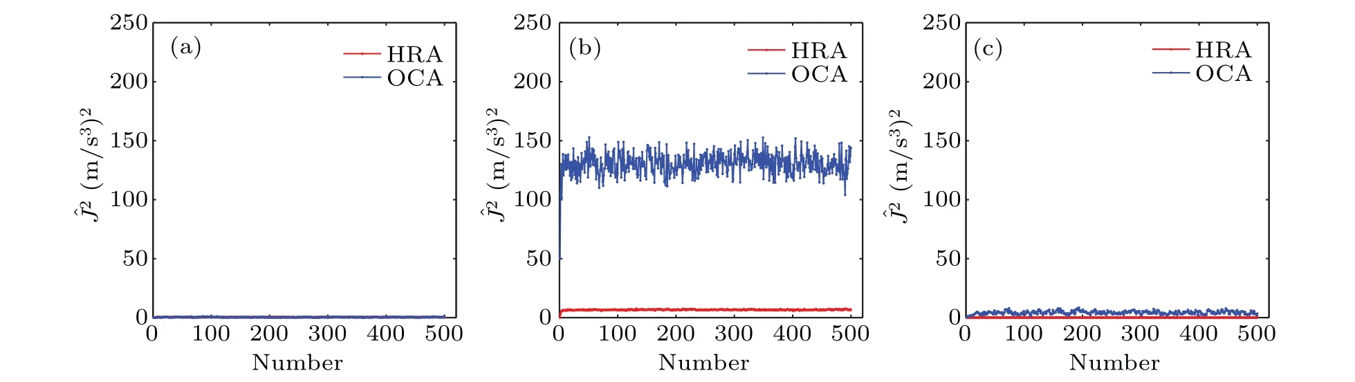
Fig.17. Comfort level(a)upstream of the control zone,(b)in the control zone,and(c)downstream of the control zone. The inflow is in low level(p0=0.06).

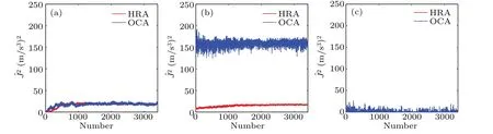
Fig.18. Comfort level (a) upstream of the control zone, (b) in the control zone, and (c) downstream of the control zone. The inflow is in medium level(p0=0.074).

Figure 16 compares the performance of HRA and OCA in terms of comfort level at the three typical levels of inflow rate.One can see that at all levels of inflow rate,driving is much more comfortable under the HRA.We also compare fuel consumption in the three road sections. As shown in Figs.17–19,the large value of ˆJ2under the OCA is mainly caused in the control zone.As one can see from panel(e)in Figs.3–5,notable jerks are mainly observed near the lane drop. The contribution of congestion to ˆJ2is not so significant because vehicles move with constant speed in the congestion. Jerks at the front of congestion region are not as strong as that near the lane drop under the OCA.

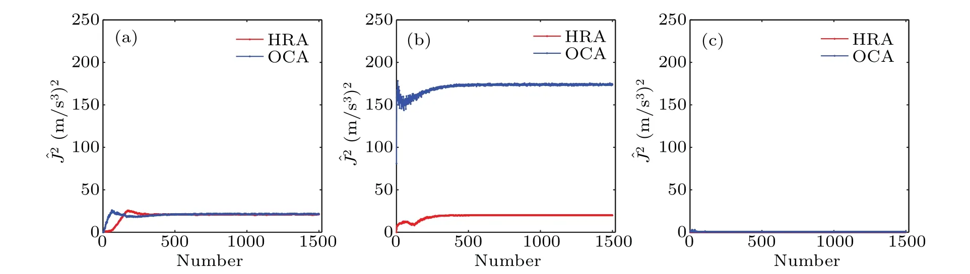
Fig.19. Comfort level(a)upstream of the control zone,(b)in the control zone,and(c)downstream of the control zone. The inflow is in high level(p0=0.09).

3.7. Sensitivity analysis

This subsection performs sensitivity analysis of the parameters,including the control gainska,kv,andkg,time gapTg,the acceleration restrictionacmd,limand safe time gapTsafe. The dependence of the capacity on the parameters is shown in Table 1.Tables 2 and 3 present the impact of the parameters on the performance metrics. The traffic flow is kept unsaturated(p0=0.06)in Table 2 and oversaturated(p0=0.09)in Table 3. The results are averaged from the 1st to the 1000th vehicle.

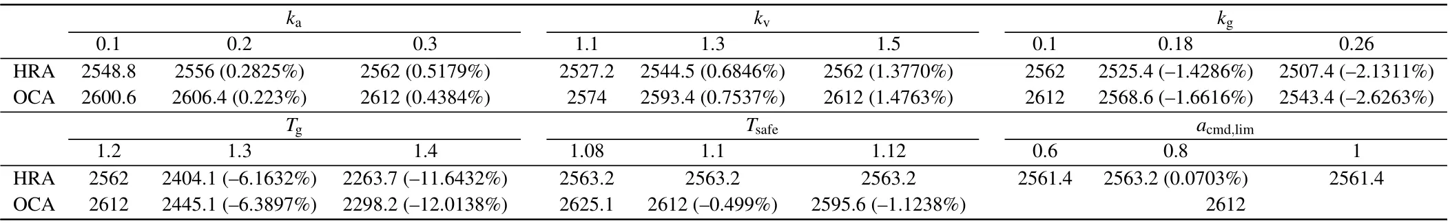
Table 1. Dependence of the capacity on the parameters.

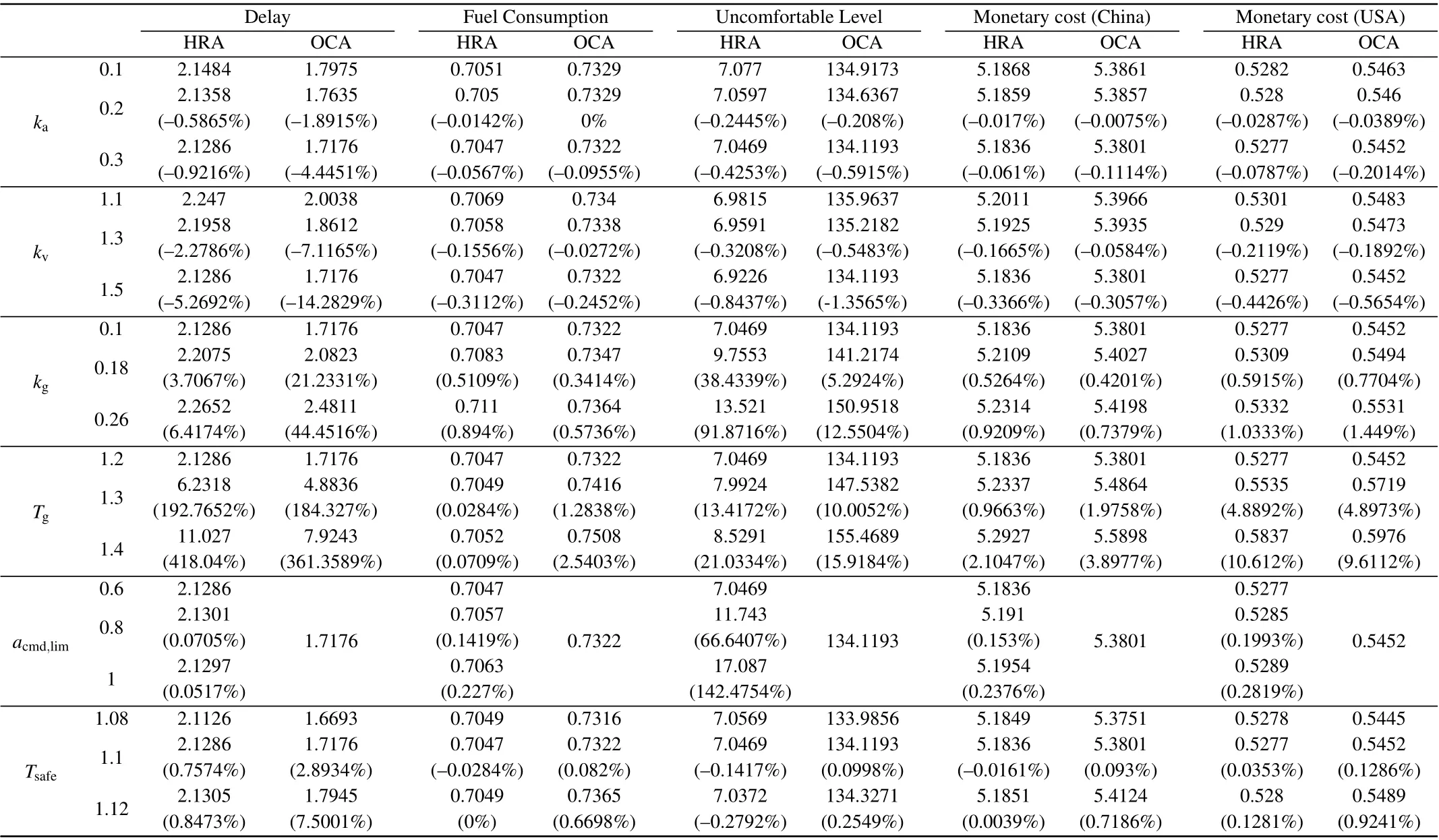
Table 2. Sensitivity analysis in the unsaturated inflow.

Table 3. Sensitivity analysis in the oversaturated inflow.

One can see thatTghas significant impact on the capacity.WhenTgincreases from 1.2 s to 1.4 s,the capacity decreases by about 11%–12%under both control algorithms. Other parameters do not have so remarkable impact on capacity.Under both control algorithms,increasingkaandkvwould slightly increase the capacity, but increasingkgwould slightly decrease the capacity. IncreasingTsafewould slightly decrease the capacity under the OCA but the impact is trivial under the HRA.Finally, the impact ofacmd,limis trivial under the HRA. Note that the OCA does not have the parameteracmd,lim.

Since increasingkaandkvhas a positive contribution to the capacity,it is expected they also could benefit the five metrics. Similarly, increasingTgandkghas a negative contribution to the capacity,thus,it is expected they also would worsen the five metrics. The results are generally as expected,as can be seen from Tables 2 and 3. Under the HRA,acmd,limhas trivial impact on the capacity as well as other four metrics.However,it has significant impact on the uncomfortable level.With the increase ofacmd,lim, the driving becomes more and more uncomfortable. Finally,since increasingTsafedecreases the capacity under the OCA, it also worsens the five metrics.Under the HRA,the impact ofTsafeon the five metrics is not significant.

4. Conclusion

There are two main approaches to deal with merging of traffic flow of CAVs. One is heuristic rules-based algorithm;the other is optimization-based control algorithm. Nevertheless,a comprehensive study on the performance of the OCAs as well as the comparison with the HRAs is lacking.

This paper evaluates the performance of a typical OCA,which maximizes the average speed of each vehicle. We also compare performance of the OCA with a HRA, in which virtual vehicle and restriction of the command acceleration caused by the virtual vehicle are introduced. We investigate the traffic flow of CAVs at lane drop on a two-lane highway.Our study found that(i)capacity under the HRA(denoted asCH)is smaller than capacity under the OCA;(ii)the travel delay is always smaller under the OCA, but driving is always much more comfortable under the HRA; (iii) when the inflow rate is smaller thanCH, the HRA outperforms the OCA with respect to the fuel consumption and the monetary cost;(iv) when the inflow rate is larger thanCH, the HRA initially performs better with respect to the fuel consumption and the monetary cost,but the OCA would become better after certain time. We present the spatiotemporal pattern and speed profile of traffic flow,which explains the reason underlying different performance of the two algorithms.

In the future work, the study can be extended in several directions. (i)Other OCAs and HRAs need to be considered.For example,acceleration might be considered in the objective function of the OCA so that trajectories can be more energy efficient. (ii) Highway with more lanes should be investigated.(iii) The on-ramp scenario needs to be studied, in which the control zone length is much shorter.(iv)The mixed traffic flow consisting of human driven vehicles should be considered.

Acknowledgements

Project supported in part by the Fundamental Research Funds for the Central Universities (Grant No. 2021JBZ107)and the National Natural Science Foundation of China(Grant Nos.72288101 and 71931002).