A Spinor Approach to the SU(2)Clebsch-Gordan Coefficients∗

2019-07-16LingDiYang杨灵迪andFaMinChen陈发敏

Communications in Theoretical Physics 2019年6期

Ling-Di Yang(杨灵迪)and Fa-Min Chen(陈发敏)

Department of Physics,Beijing Jiaotong University,Beijing 100044,China

AbstractWe review the irreducible representation of an angular momentum vector operator constructed in terms of spinor algebra.We generalize the idea of spinor approach to study the coupling of the eigenstates of two independent angular momentum vector operators.Utilizing the spinor algebra,we are able to develop a simple way for calculating the SU(2)Clebsch-Gordan(CG)coefficients.The explicit expression for the SU(2)CG coefficients is worked out,and some simple physical examples are presented to illustrate the spinor approach.

Key words:Clebsch-Gordan coefficients,spinors,representations

1 Introduction

It is well known that the finite dimensional(irreducible)representation of an angular momentum vector operator can be constructed by employing a pair of spinors.[1−2]The CG coefficients1couple the individual eigenstates of two independent angular momentum operators J1and J2to form the eigenstates of the total angular momentum operator J=J1+J2.So,if we use two independent pairs of spinors to construct the individual states of J1and J2,and take care of the coupling of these two pairs of spinors,it is possible to work out the CG coefficients.Our goal is to derive all CG coefficients using this spinor approach.It seems that this approach is simpler than the conventional approaches[5−6]for calculating the CG coefficients.

This paper is organized as follows.In Sec.2,we briefly review the irreducible representation of the set of SU(2)generators or angular momentum vector operator using the spinor approach.The reader who is familiar with it may skip this section.In Sec.3,we present our detailed calculations on CG coefficients utilizing the spinor algebra.In Sec.4,we work out some simple physical examples to illustrate the spinor approach.Section 5 is devoted to discussions.In Appendix A,we sketch two conventional methods for calculating the SU(2)CG coefficients.

2 Review of Representation of SU(2)

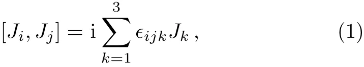
In this section,we briefly review the spinor construction of the irreducible representation of the Lie algebra of SU(2).[1]The three generators of SU(2)or the components of angular momentum J satisfy the usual commutation relation2

We denote the “spin up” and “spin down” spinors as ξ1and ξ2,respectively.The action of Jion ξα(α =1,2)is as follows

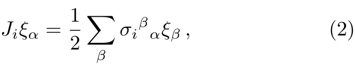
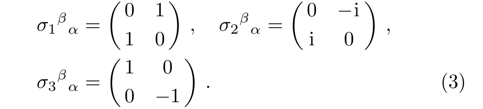
And the Leibnitz rule

is assumed.Equation(2)is equivalent to

where J±=J1±iJ2or Jx±iJyare the usual raising and lowering operators.

The(irreducible)(2j+1)-dimensional representation of Jican be constructed by introducing the set of basis state vectors

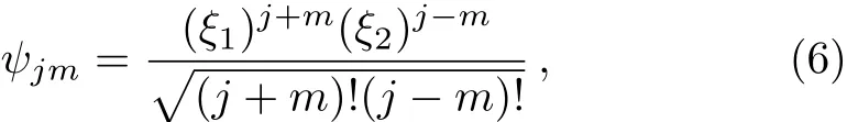
with j=0,1/2,1,3/2,2,...,and m= −j,−j+1,...,j−1,j.The physical interpretation of Eq.(6)is that it describes a state of 2j spin 1/2 particles;specifically,it describes the state of(j+m)“spin up” particles and(j−m)“spin down”particles.Using Eqs.(2)and(4),we see that the corresponding eigenvalues of J2and J3are j(j+1)and m,respectively,i.e.,

and it is easy to show that

The irreducible representation matricesdefined bycan be read o fffrom Eqs.(7)and(8).By Eq.(8),we see that the matrix elements ofare real and positive3If we use the following “τ-pauli” matricesto replace the σ-pauli matrices in Eqs.(2)and(3),Eqs.(7)remain unchanged,but the matrix elements(9)turn out to However,we follow the convention of Refs.[5–7]by setting the phase factor eiδ =1.,i.e.,

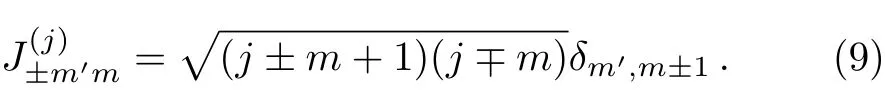
Also,the matrix elements of the raising and lowering operators defined via Eqs.(14),(15),and(40)are real and positive.

3 SU(2)CG Coefficients and Spinors

We now consider two independent angular momentum vector operators J1and J2and their coupling.Following the idea of the last section,it is not difficult to construct the simultaneous eigenstate of J21,J22,J1z,and J2z:

Here ηαis another independent pair of spinors.The action of J1and J2on the spinors is as follows

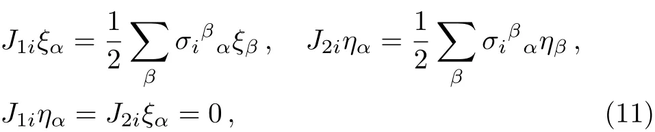
and the Leibnitz rule,similar to Eq.(4),is assumed.We see that Eq.(10)is an obvious generalization of Eq.(6).In summary,the state vector ψj1j2;m1m2satisfies

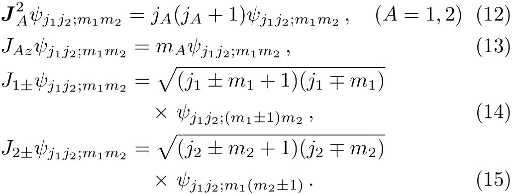
Here JA±=JAx±iJAy.Notice that ψj1j2;m1m2is also an eigenstate of Jz=J1z+J2z,the z-component of the total angular momentum

It is useful to consider the general SU(2)transformation generated by J.It can be defined as follows.Let U=exp(iθ ·J),where θ is a vector of parameters.Using Eq.(11),we learn that

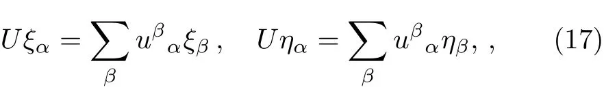
where uβα= (eiθ·σ/2)βα,obeying u†u = 12×2and detu=1,namely

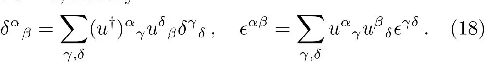
Here ϵαβ(ϵ12= −ϵ21= −1)is the antisymmetric tensor.Later we will see that ϵαβplays the key role for constructing the eigenstates of the total angular momentum.

Our central task is to construct the general eigenstate ψj1j2;jmof J21,J22,J2,and Jz,as a linear superposition of ψj1j2;m1m2,

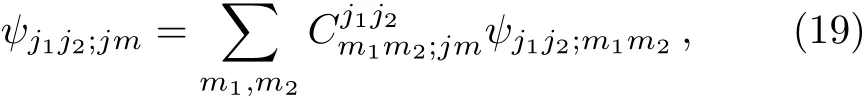
and read o ffthe CG coefficients from the above unitary transformation.As usual,we use j and m to label the quantum numbers of J2and Jz,respectively.

The basic strategy is to construct ψj1j2;jjfirst,with|j2−j1|≤j≤j1+j2,then use the lowering operator J−=J1−+J2−to act on it(j − m)times to get the general state ψj1j2;jm.

We begin by considering the special case j1=j2.In this case,the minimum j is 0.The essential observation is that the state ψj1j1;j=0,m=0must take the following form:

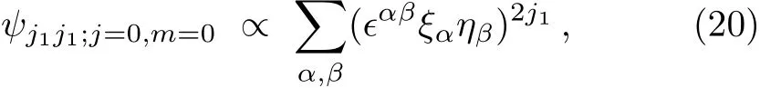
(up to a normalization constant).In fact,due to the constraint of the antisymmetric tensor ϵαβ,the number of“spin up” particles is exactly the same as the number of“spin down”particles,so Eq.(20)must be the spin zero state of the total angular momentum J;Or in other words,due to the second equation of Eqs.(18),(20)must transform as a scalar under the SU(2)transformation(17).This can be proved as follows:Using

and Eq.(11),a short calculation gives

Taking account of the equation

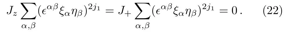
we see that it is indeed the spin zero state,namely,

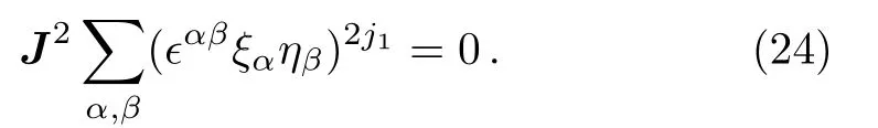
Finally,notice that Eq.(20)is also the simultaneous eigenstate of J21and J22,belonging to the same eigenvalue j1(j1+1).This completes the proof.The next step is to construct ψj1j1;j=1,m=1;it must take the following form:

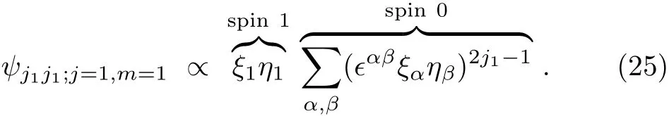
More generally

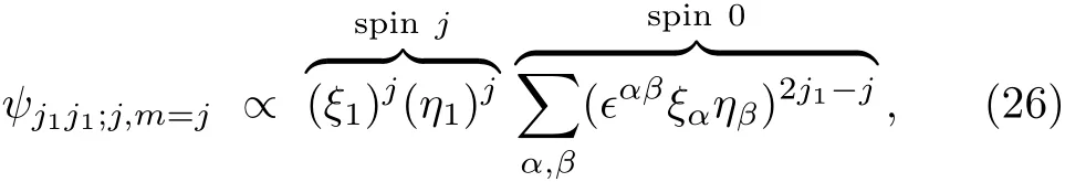
where 0≤j≤j1+j2=2j1.We are going to prove Eq.(26)a little later.

We are now ready to construct ψj1j1;jj,without assuming j1=j2.Following the idea for constructing Eqs.(20)and(26),it is natural to propose4Similarly,one may construct ψj1j2;j(−j)as follows:

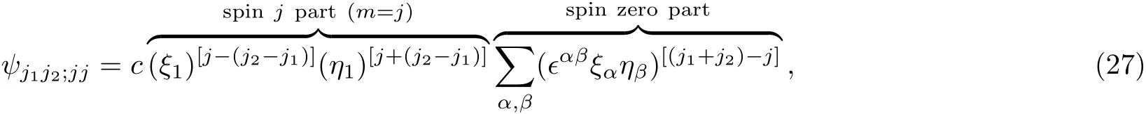
with c a constant.If j1=j2,Eq.(27)is reduced to Eq.(26);So it is sufficient to prove Eq.(27).In Eq.(27),the part constrained by the antisymmetric tensor ϵαβis obviously the “spin zero” part,while the rest part,containing[j−(j2−j1)]+[j+(j2−j1)]=2j“spin up”particles,must be the“spin j”part with m=j.It is not difficult to prove this claim:Using Eqs.(21)and(11),we see immediately that the right-hand side of Eq.(27)is annihilated by J+,

while it is an eigenstate of Jz,belonging to the eigenvalue j,

On account of Eq.(23),we learn that the right-hand side of Eq.(27)is indeed the eigenstate of J2,and the corresponding eigenvalue is j(j+1).

On other hand,in Eq.(27),we have 2j1ξ-type spinors and 2j2η-type spinors,so Eq.(27)must be the simultaneous eigenstate of J21and J22.To see this,let us expand the right-hand side of Eq.(27):

Using Eq.(10),the above expression can be converted into

In the second line,we have set j1−r=m1and m2=j−j1+r;And

is the normalization constant,to be given by Eq.(37).Now it is manifest that the second line of Eq.(31)is the simultaneous eigenstate of J21,J22,and Jz,and the corresponding eigenvalues are j1(j1+1),j2(j2+1),and m1+m2,respectively.

The range of j can be determined by noting that the powers of the spinors in Eq.(27)must be non-negative integers,i.e.,

which are nothing but

which can be evaluated using the identity5It can be proved by Taylor expanding the equation(x+y)−n(x+y)−m=(x+y)−(n+m),where m and n are positive real numbers.

where ni≥0(i=1,2,3).A short computation gives

with eiγthe phase factor;We choose our phase convention by setting

i.e.,the normalization constant c of Eq.(27)depends on the sign of(−1)j1+j2−j.

Now the general state ψj1j2;jmcan be worked out in the standard way.Using the lower sign of the equations

we learn that

Using Eq.(14),we learn that

and(J2−)j−m−rψj1j2;m1m2has a similar expression.Substituting Eqs.(31),(37),and(42)into Eq.(41),and relabeling the indices,then comparing the expression with Eq.(19),we obtain

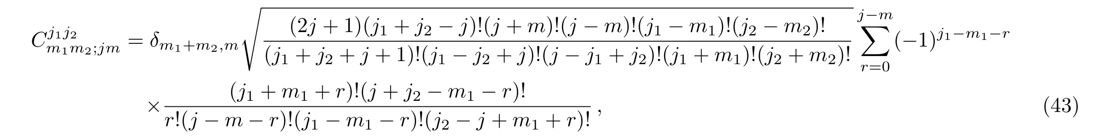
which is in agreement with the result in Ref.[7].

Let us comment on our phase convention.With the choice of phase factor(38),our phase convention is identical with that of Ref.[7].In Ref.[7],the phase factor of ψj1j2;jjis fixed by requiring that

The above two requirements are equivalent(see Sec.3.4 and 3.5 of Ref.[7]). One can easily read o ff ourfrom Eq.(31):

which is obviously positive.

We see that using the antisymmetric tensor ϵαβproperly,we have been able to construct ψj1j2;jjin terms of ψj1j2;m1m2with very little calculations(see Eqs.(27)and(31)),leading to a simple calculation of the explicit expression of CG coefficients(43).However,in the most conventional approach,[5]it is not that easy to construct ψj1j2;jjwhen j=j1+j2:One has to work out ψj1j2;(j1+j2)(j1+j2),ψj1j2;(j1+j2−1)(j1+j2−1),...,and ψj1j2;|j1−j2||j1−j2|step by step7Alternatively,one has to work out ψj1j2;(j1+j2)(−j1−j2), ψj1j2;(j1+j2−1)(−j1−j2+1),...,and ψj1j2;|j1−j2|(−|j1−j2|)step by step..

In another conventional approach,[6]the strategy is to derive recursion relations for the CG coefficients.Using the recursion relations and the normalization conditions of CG coefficients,in principle one can work out all nonvanishing CG coefficients.However,the calculation is so involved that the textbook[6]says that“With enough patience we can obtain the Clebsch-Gordan coefficient of every site in terms of the coefficient of the starting site,A.”

In summary,it is not that simple to use the conventional approaches to work out the general expression of the SU(2)CG coefficients(43).See Appendix A for a quick review for these two conventional methods of computing the CG coefficients.

4 Simple Physical Examples

In this section,we work out some simple physical examples using the method developed in Sec.3.We begin by considering the familiar case of the coupling of two spin 1/2 particles,such as two electrons.For j1=j2=1/2,according to Eq.(34),j has two possible values:1 or 0.If j=0,using Eq.(20)or Eq.(27),we obtain the spin singlet

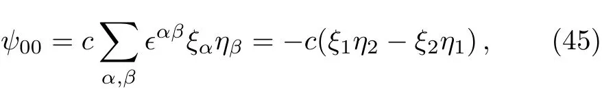
immediately.Here we have omitted the quantum numbers j1and j2.By Eqs.(37)–(39),the normalization constant is c= −1Following the convention of Ref.[6],we will use “±” to denote “spin up” and “spin down”,respectively.defining ψ1+≡ ξ1,ψ1−≡ ξ2,ψ2+≡ η1,and ψ2−≡ η2,the singlet Eq.(45)takes the familiar form,

Also,using Eq.(27),we learn that the spin triplet with quantum numbers j=m=1 takes the following form(the normalization constant c is obviously equal to 1):

And the rest state vectors of spin triplet can be determined in the standard way Eq.(41);For instance,

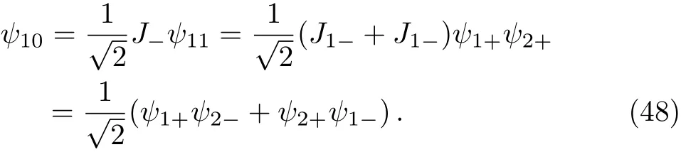
Similarly,

It is a simple matter to read o ffthe CG coefficients from the above equations.

We now turn to the case of j1=j2=1,i.e.,the coupling of two identical spin 1 particles.According to Eq.(34),j=0,1,or 2.If j=0,using Eqs.(27)and(10),or using Eq.(31)directly,we obtain

By Eqs.(37)–(39),the normalization constant is2c=Comparing the above equation with Eq.(19)determines the corresponding CG coefficients:

which are in agreement with the results in the textbook.[5]Similarly,by Eqs.(27)and(10),or Eq.(31),we have

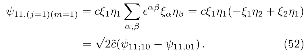
The normalization constant can be determined by using Eqs.(37)–(39);It is˜c=−c=1/2 by Eqs.(37)–(39).And

where the normalization constant c is 1/2 by our convention defined by Eqs.(37)–(39). One can use the standard way(41)to work out ψ11,(j=1)(m=0,−1)and ψ11,(j=2)(m=0,±1,−2),and read o ff the CG coefficients.Since these calculations are quite standard and straightforward,we do not present them here.

Since the quantum numbers discussed in this section are small(j1=j2=1/2 or j1=j2=1),it is also not difficult to work out the coupling of(spin)state vectors of two identical particles by using the conventional approaches described in Appendix A.However,for arbitrary j1and j2,the spinor approach for working out the general expression(43)of CG coefficients is more convenient and efficient.

5 Discussions

In summary,we have derived the expression of SU(2)CG coefficients coupling two independent angular momentum vector operators utilizing the spinor algebra,and presented two simple physical examples to illustrate the spinor approach.Clearly,one can generalize this spinor approach to work out the expressions for 6j and 9j coefficients coupling three and four angular momentum vector operators,respectively.

Appendix A:Sketches of Conventional Calculations of SU(2)CG Coefficients

In this appendix,we briefly sketch the two conventional methods for calculating the SU(2)CG coefficients in Refs.[5]and[6],respectively.In Refs.[5–6],the overall phase factor for the CG coefficients is not specified;We shall fix the phase factor by adopting the convention of Ref.[7](see(44)).

In the most conventional approach to CG coefficients,say for example,in Ref.[5],the first step is to assume that both j and m take the maximum value j=j1+j2=m and to construct the state vector8For convenience,we still use ψ to denote the wave functions,though they do not necessarily take exactly the same forms as that of(6)and(10).

The only CG coefficient is

where we have fixed the phase factor by using the convention Eq.(44).Evaluating the following equation

gives

Comparing the above equation with Eq.(19),one can read o ffthe corresponding CG coefficients. Similarly, one can obtain ψj1j2;(j1+j2)mby evaluating(J−)(j1+j2)−mψj1j2;(j1+j2)(j1+j2),and then one can read of the CG coefficients

The next step is to consider

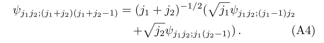
The state vector ψj1j2;(j1+j2−1)(j1+j2−1)must be orthogonal to ψj1j2;(j1+j2)(j1+j2−1).(Recall that J2is a hermitian operator,so its two eigenstates corresponding to two different eigenvalues must be orthogonal.)Equation(A4)suggests that

Let us fix above overall phase factor eiδby using the convention(44).Comparing Eq.(A6)with Eq.(19),we can read off the CG coefficient

Comparing(A7)with(44)determines the phase factor eiδ=1.However,in Ref.[5],the phase factor in Eq.(59)is eiδ= −1.This is not a problem:According to chapter 4 of Ref.[5],the state vector Eq.(A6)is defined“apart from an arbitrary choice of a phase factor”.

One then derives ψj1j2;(j1+j2−1)mby calculating(J−)(j1+j2−1)−mψj1j2;(j1+j2−1)(j1+j2−1),and read of the CG coefficients

Similarly,one can construct

by noting that it must be orthogonalto both ψj1j2;(j1+j2−1)(j1+j2−2)and ψj1j2;(j1+j2)(j1+j2−2);And the overall phase factor can be fixed by using the convention(44).Then one can derive ψj1j2;(j1+j2−2)mby using the lowering operator J−to act on Eq.(A8)[(j1+j2−2)−m]times.

Continuing in this way until j reaches the minimum value j=|j1−j2|,one can work out all CG coefficients in principle.However,the calculation for working out the general expression of SU(2)CG coefficients(43)is lengthy and complicated.

Another conventional way is based on the recursion relations for CG coefficients.[6]We now briefly outline this method.For simplicity,we will omit the quantum numbers j1j2;For instance,we will write|j1j2;jm＞as|jm＞.The recursion relations can be derived by calculating the matrix elements

in two different ways.Using(J1±+J2±)=(J†1∓+J†2∓),a short computation gives the recursion relations:

In terms of our notation,the CG coefficients read

The textbook[6]derives Eq.(63)in a slightly different way.Similarly,by evaluating the matrix elements

we obtain conditions for non-vanishing CG coefficients

The recursion relations(A10)and the normalization conditions

determine all CG coefficients(up to an overall phase factor).To see this,we consider the lower signs of Eq.(A10).Note that if we set m1=j1,the first term of the right-hand side of Eq.(A10)vanishes,i.e.,

For convenience,we use “A” and “B” to stand for ＜j1(m2+1)|jm＞and ＜j1m2|j(m − 1)＞,respectively9They are the CG coefficients in the sites“A”and“B”of Fig.3.9 of Ref.[6]..We see that“B” can be expressed in terms of“A”.Here we treat“A” as a starting coefficient.Later we will see,the rest of CG coefficients can be expressed in terms of“A”as well.For instance,if we take the upper signs of Eq.(A10),and do the replacements:

Eq.(A10)becomes

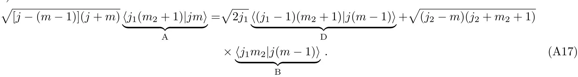
Here the key point is that we have used“A”and “B”to generate a new CG coefficient“D”.By Eqs.(A15)and(A17),we see that“D” can be also expressed in terms of“A”.

• Similarly,we can use“B” and “D” to generate a new CG coefficient“E”,and express“E” in terms of“A”;

• And then it is possible to use“B” and “E” to generate a new CG coefficient“C”,and express“C” in terms of“A”.

Continuing in this way,with “enough patience”,as the textbook[6]pointed out,we can express the rest of CG coefficients in terms of the CG coefficient“A”.And the CG coefficient“A”can be determined(up to an overall phase factor)by the normalization conditions(A14).However,the calculation is quite involved,as the textbook[6]noticed.

We shall fix the overall phase factor by adopting the convention(44).In Eq.(A15),if we set m=j,and replace m2+1 by m2,then CG coefficient “A” reads ＜j1m2|jj＞.According to Eq.(44),it satisfies

namely,the above overall phase factor is eiδ=1.

For more detailed discussions and calculations of the CG coefficients using the approach of recursion relations,see Refs.[6]and[7].

Acknowledgement

We are grateful to Yan-Wu Lu for useful discussions.

Communications in Theoretical Physics

2019年6期