Thad Michael , Jianming Yang , Frederick Stern

1. NSWC Carderock Division, 9500 MacArthur Blvd., West Bethesda, MD 20817, USA,E-mail:thad.michael@navy.mil

2. Fidesi Solutions LLC, PO Box 734, Iowa City, IA 52244, USA

3. IIHR-Hydroscience and Engineering, University of Iowa, Iowa City, IA 52242, USA

Introduction

Cavitation is the term for the change of state from liquid to vapor when it is caused by a lowpressure region within the flow field at an ambient temperature. Although the physical mechanism is the same, in contrast the term boiling is used to describe the change of state from liquid to vapor when it is caused by a local increase in temperature at the ambient pressure. For cavitation, the phase change rate is governed by the local pressure, while for boiling it is governed by the local temperature.

Cavitation degrades the performance of lifting surfaces found on ships, such as propeller blades and rudders. In addition to reducing lift, the violent collapse of cavitation bubbles can also remove material leading to further degradation and possible failure.

Potential flow cavitation models have been developed for propellers in Refs.[1,2]. The cavity is treated as additional thickness and the location is solved iteratively. A number of cavitation models for viscous flows have been developed, primarily for homogenous mixture models. Some examples are Refs.[3,4]. A more recent model in Ref.[5] adds the effect of noncondensable gas within the bubbles. Recent computations in Refs.[6-9] using models of this type have compared well with hydrofoil experiments. For visualization, the cavity interface is assumed to be at a constant volume fraction, typically 0.5. For summaries of recent research on cavitation models, especially,homogeneous mixture models, and their applications,the reader is referred to [10-13].

Sharp interface phase change models have been used to compute film boiling in Refs.[14,15]. Here we seek to apply similar techniques to the problem of cavitation, with the development of a suitable model for phase change due to cavitation.

The focus of this paper is the development of a model for predicting the phase change rate suitable for use with a sharp interface and the necessary models and methods to support this combination. The model is implemented in a two-phase incompressible viscous flow solver with a sharp interface approach. Results are presented for a cavitating hydrofoil. The results are analyzed to reveal details of the physics of the reentrant jet and cavity shedding. The averaged results are compared with experimental data.

1. Mathematical model

1.1 Incompressible viscous flow

The Navier-Stokes equations for the incompressible viscous flow of the liquid and vapor phases are written as follows:

where I is the identity matrix and where μ is the viscosity of the fluid and

1.2 Phase change

With phase change, a volume source must be added due to the different densities of liquid and vapor.The volume source satisfies the requirement for mass conservation and results in a jump in the fluid velocity at the interface so that Eq.(1) becomes

where m˙ is the mass flux between phases and the subscripts l and v stand for liquid and vapor, respectively.

1.3 Interface tracking

A volume of fluid (VOF) method described in Ref.[16] with the addition of a velocity component due to phase change is used to track the interface position. Without phase change, the boundary between liquid and vapor moves with a velocity which is continuous across the interface. Phase change introduces a velocity discontinuity at the interface which is proportional to the phase change rate and the difference in density across the interface. The VOF equation is

where U is the interface velocity, defined relative to the local liquid or vapor velocity by

wherefu is the fluid velocity, and ρfis the fluid density and f is liquid or vapor. This satisfies the conservation of mass between the phases at the interface.

1.4 Modeling mass flux between phases

The rates of vaporization and condensation are determined by a simplification of the Rayleigh-Plesset equation which assumes a spherical bubble subject to uniform pressure variations wherevapp is the vapor pressure,0gp is the initial partial pressure of non-condensable gasses,0R is the initial radius of the bubble, S is the surface tension,and γ is the ratio of the gas heat capacities. The third term on the right-hand side represents the effect of the non-condensable gasses. The last two terms on the right represent the effects of surface tension and viscosity, respectively.

The surface tension can be neglected for all but the smallest bubbles and the viscous effects can be neglected for the Reynolds numbers of interest in ship flows. By also neglecting the non-condensable gasses,the equation can be integrated with respect to time and simplified to yield

This simplification is the foundation of several cavitation models used with two-phase mixture models where further assumptions about bubble number or size are utilized to arrive at a surface area and mass flux.

With a sharp interface method, the bubble must be larger than the cell to be accurately modeled. If the radius is sufficiently large, it is reasonable to represent it by a plane within the cell, as in the volume of fluid method. Then, the velocity is

where n is the interface normal. Because a local pressure will be used in place of the far field pressure,a constant is needed for correlation. With this addition,and a simplification, the mass flux can be expressed:

whereeC andcC are the coefficients of evaporation and condensation, respectively. See Ref.[17] for a more detailed derivation.

2. Numerical methods

2.1 Flow solver

The CFD code CFDShip-Iowa v6.2[18]is the foundation for this development. It is an incompressible Navier-Stokes solver utilizing an orthogonal curvilinear grid. The velocity components are defined at the centers of cell faces while other quantities are defined at the cell centers. A finite difference approach is used, except for the pressure Poisson equation which is solved with a finite volume approach. For cavitation modeling, a first-order Euler method is used for time advancement for simplicity.

Hypre library[19]is used for the parallel solution of the Poisson equation. With the volume source due to phase change, the Poisson equation is

where G radi(p) is collocated with the velocity components and incorporates the jump conditions due to surface tension and gravity as described in Ref.[20].For stability, the phase change rate from Eq.(11) is modeled semi-implicitly, as described in Ref.[17],resulting in this pressure Poisson equation

where E is a constant related to the fluid densities

For the momentum equation, a ghost fluid method is employed. This method was also used in Refs.[14,15] to model boiling with a sharp interface phase change model. CFDShip-Iowa v6.2 includes surface tension, density, and viscosity changes at the interface[20]. The ghost fluid method is used only to account for the velocity jump normal to the interface due to the volume source.

Fig.1 Hydrofoil geometry with six-degree angle-of-attack

Fig.2 Leading edge of the foil and grid resolution

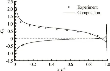
Fig.3 Pressure distribution on the foil without cavitation, 2-D calculation. Experimental data is from Ref.[23]

A parallel fast marching method developed in Ref.[21] was also modified to extend the velocity components from one side of the interface to the other such that the velocity normal to the interface is constant. The extended velocity field is not conservative. However, only the extended values that are close to the interface are used to solve the momentum equation in the phase of interest and the approximation is reasonable near the interface. The momentum equation is solved separately for each phase and the intermediate velocity fields are then combined using the level set function to discriminate between phases.

Fig.4 (Color online) Cavity evolution at 1.25 cavitation number (p = - 0 .625), time series from a-h

2.2 Volume of fluid and level set

The VOF method is used for interface reconstruction and advection as described in Ref.[16]. An operator splitting strategy is used to advect the interface separately in each coordinate direction. The velocity used for VOF advection is the interface velocity field computed by applying Eq.(11) to the two-phase velocity field.

The level set scalar is reinitialized from the VOF using a parallel fast marching method described in Ref.[21].

2.3 Interface area and location

In the earlier implementation of this cavitation model described in Ref.[17], some discrepancies arose between the definition of the interface location used for the ghost fluid method and the volume source.The ghost fluid velocity extension utilizes the level set function interpolated to the face centers where the ve-locity is defined. Previously, the volume source was determined by the interface area from the VOF interface reconstruction. However, the two methods could lead to contradictions when the interface was close to a cell face.

Fig.5 (Color online) Cavity trailing edge showing stagnation point and reentrant jet

Fig.6 (Color online) Middle of cavity showing bulge where reentrant jet begins to push outward into cavity. (For clarity, vectors are only shown at every other point.)

To eliminate this problem, a marching cubes method has been implemented following the method in Ref.[22]. By interpolating the level set function from cell centers to face centers, edge centers, and corners, a triangulated surface is obtained which is consistent with the interface used for the velocity extension in the ghost fluid method. The interface area can then be determined directly from the area of the triangles in each cell and used in the finite volume implementation of the pressure Poisson equation with a volume source. The triangulated surface is also useful for visualization.

3. Results and discussion

3.1 Two dimensions

Previous computations with simple 2-D bubble cases showed that the velocity jump is well represented and the pressure and velocity distributions around the bubble follow the analytical solutions[17].

Computations have been made for a hydrofoil tested in Ref.[23]. The thickness of the hydrofoil is 9%of the chord length with a NACA 66 distribution. The camber is 2% of the chord length with a NACA a = 0.8 distribution. In the experiment, the span of the foil was equal to the chord. The angle-of-attack is 6o.

Here, a 2-D slice of the foil is modeled with an O-grid with 2 048 cells wrapping around the foil and 256 cells in the surface normal direction. The radius of the O-grid is about 10 chord lengths. Upstream, the inlet velocity is specified. Downstream, the pressure is specified. The geometry is shown in Fig.1 and Fig.2 shows a detail of the mesh near the leading edge.

The cells near the surface of the foil are approximately square and approximately constant size. The fixed resolution is important to accurately capture the bubbles.

A calculation without cavitation verifies the pressure distribution is accurately predicted on the foil,as shown in Fig.3. The computed lift coefficient of 0.824 is 3.3% greater than the experiment6ally measured value at the Reynolds number of 2×10.

With the cavitation number set to 1.25 to match the experiment, a time series of the initial cavity development is shown in Fig.4. Note that the contour legend shown in Fig.4 applies to all figures with pressure contours and that p in the figures is normalized with ρ U2. so that the vapor pressure is p=-0 .625. The sequence shows that as the cavity grows downstream, a thin layer of liquid remains on the foil surface. This is because the downstream growth of the cavity is driven mainly by advection and there is a no-slip condition on the surface of the foil.

The stagnation point at the downstream end of the cavity causes a high pressure at that location which tends to force liquid back upstream, underneath the cavity, as shown in Fig.5. This flow characteristic is often called the reentrant jet.

As shown in Fig.5, the vapor flow at the outer surface of the cavity follows the liquid flow on the other side of the interface downstream. Drops of liquid from under the cavity are carried downstream and collect in the downstream portion of the cavity.

A short distance from the stagnation point, the pressure in and under the cavity is equal and the liquid under the cavity can easily find its way into the cavity,as shown in Fig.6.

Figure 7 shows a time series near the middle of the cavity. The liquid under the cavity is pushed up into the cavity by the flow of the reentrant jet from downstream (a, b). As the finger of liquid approaches and touches the outer surface of the cavity, it is drawn downstream (c, d), stretches (e, f) and breaks up into separate regions (g, h).

Fig.7 (Color online) Reentrant jet flow under and into cavity, time series from a-h

If sufficient liquid collects in the downstream end of the cavity, or if a finger of liquid from the reentrant jet destabilizes the cavity enough to allow a high pressure to develop between the upstream and downstream portions of the cavity, the downstream portion of the cavity will be shed downstream and will gradually disappear as the vapor becomes liquid again.

The current model does not capture the effect of the non-condensable gasses that diffuse into the cavity and will remain in the bubble after the vapor becomes liquid again.

Figure 8 is a time sequence showing the flow field where, qualitatively, the downstream portion of the cavity begins to separate from the upstream portion before moving downstream while the upstream cavity sheds some additional vapor regions and shrinks. There is no sudden shift in the flow patterns.It appears that liquid accumulates under and among the cavities until the liquid displaces the cavities sufficiently high into the flow field for them to be swept downstream.

Following shedding, the development of the new cavity is more complex than the initial development shown in Fig.4. There is not a single vapor-filled cavity, but instead a group of them occupying a similar extent to that shown in Fig,4(h) and Fig.8. The physical processes appear to be similar, including the recirculation or the reentrant jet and increasing liquid fraction.

Fig.8 (Color online) Shedding. The first image is an overview of the cavity shape at shedding, the arrow indicates the location shown in the other images. The other images show the flow at the point where shedding appears to initiate at times just before, during, and after shedding

Fig.9 Grid near foil leading edge. The similar discretization in all three directions is important for capturing bubbles with a sharp interface method

Fig.10 Pressure distribution on the foil without cavitation, 3-D calculation averaged across span. Experimental data is from Ref.[23]

3.2 Three dimensions

The same hydrofoil is modeled in three dimensions with an O-grid of 1 024 cells wrapping around the foil, 1 024 cells in the spanwise direction, and 128 cells in the surface normal direction. In the area of interest near the foil surface on the suction side, the cells are approximately cubes. The surface grid near the foil leading edge and a cut through the grid in a plane normal to the span is shown in Fig.9.

Fig.11 (Color online) Inception bubbles near the leading edge of the foil

Three calculations have been made: (1) the non-cavitating foil, (2) the cavitating foil initialized with a 2-D cavitating solution, and (3) the cavitating foil from inception.

Fig.12 (Color online) Close up of inception bubbles near the leading edge of the foil

Fig.13 (Color online) Close up near the leading edge of the foil showing bubble growth, merging, and advection

As expected, the non-cavitating 3-D pressure distribution is similar to the 2-D wetted pressure distribution. However, there are some variations due to the fineness of the grid. The fine grid results in a DNS-like unsteady behavior, with vortices shed from the leading edge on the suction side. Averaging over the span of the foil shows the expected results, shown in Fig.10.

A 3-D cavitating calculation has been initiated.Figures 11 through 13 show cavitation inception near the leading edge of the foil. The inception model generates a bubble of fixed radius, large enough to include several cells. The bubbles are then free to evolve and merge. It is clear from the calculations that the evolution of the bubbles is dominated by advection.

The pattern in the initial spanwise spacing,clearly visible in Fig.12, is due to one of the criteria in the inception model. The inception model requires that the center of a new bubble be a bit more than one radius from the nearest interface. Consequently, the model tends to create a line of bubbles along the low-pressure region at the leading edge.

Only the initial startup of the 3-D calculation has been completed. As the bubbles stretch, break up, and interact with others, it is found that the stability of the computation is affected. A major reason might be the under-resolved bubbles generated in the process. A bubble model may be required to improve the numerical stability. On the other hand, Refs.[24,25] proposed a multi-scale approach to smoothly bridge large size cavities captured by level sets and small bubbles described by a discrete singularity model. Future work will require a closer look into similar models.

4. conclusions

A sharp interface cavitation model has been developed and implemented. The method utilizes a simplification of the Rayleigh-Plesset equation to compute the interface velocity used to advect the interface between the liquid and vapor phases.

The method has been demonstrated in two dimensions with a hydrofoil and found to offer insight into the mechanism of cavity evolution. The results show the formation of the reentrant jet and how instabilities in the reentrant jet perturb the cavity.Increasing liquid content, particularly near the leading edge of the cavity seems to gradually lead to cavity shedding.

The method in three dimensions has proved to be more challenging. Of course, complex geometries and moving boundaries in 3-D will pose additional difficulties to the current approach with the orthogonal curvilinear grid requirement. It is believed that together with unstructured mesh approaches or immersed boundary approaches[26]this method will lead to viable high-fidelity cavitation calculations in the near future.

This research was supported by the NSWC Carderock ILIR program and by the US Office of Naval Research (Grant No. N000141-01-00-1-7), with Dr. Ki-Han Kim as the program manager. The computations were performed on computers at AFRL and Navy DoD Supercomputing Resource Centers.

[1] Lee C. S. Prediction of steady and unsteady performance of marine propellers with or without cavitation by numerical lifting surface theory [D]. Doctoral Thesis, Cambridge,Massachusetts, USA: Massachusetts Institute of Technology, 1979.

[2] Kerwin J. E., Kinnas S. A., Lee J. T. et al. A surface panel method for the hydrodynamic analysis of ducted propellers [J]. SNAME Transactions, 1987, 95: 93-122.

[3] Merkle C. L., Feng J. Z., Buelow P. E. O. Computational modeling of the dynamics of sheet cavitation [C]. Third International Symposium on Cavitation. Grenoble, France,1998.

[4] Kunz R. F., Boger D. A., Chyczewski T. S. et al. Multiphase CFD analysis of natural and ventilated cavitation about submerged bodies [C]. Proceedings of FEDSM ’99,3rd ASME/JSME Joint Fluids Engineering Conference.San Francisco, California, USA, 1999.

[5] Singhal A. K., Athavale M. M., Li H. et al. Mathematical basis and validation of the full cavitation model [J].Journal of Fluids Engineering, 2002, 124(3): 617-624.

[6] Kim S. E., Brewton S. A multiphase approach to turbulent cavitating flows [C]. Proceedings of the 27th Symposium on Naval Hydrodynamics. Seoul, Korea, 2008.

[7] Kim S. E., Schroeder S., Jasak H. A multi-phase CFD framework for predicting performance of marine propulsors [C]. The 13th International Symposium on Transport Phenomena and Dynamics of Rotating Machinery.Honolulu, Hawaii, USA, 2010.

[8] Kim S. E., Schroeder S. Numerical study of thrust-breakdown due to cavitation on a hydrofoil, a propeller, and a waterjet [C]. Proceedings of the 28th Symposium on Naval Hydrodynamics. Pasedena, California, USA, 2010.

[9] Bensow R. E., Huuva T., Bark G. Large eddy simulation of cavitating propeller flows [C]. 27th Symposium on Naval Hydrodynamics. Seoul, Korea, 2008.

[10] Zhang, L. X., Zhang N., Peng X. X. et al. A review of studies of mechanism and prediction of tip vortex cavitation inception [J]. Journal of Hydrodynamics, 2015, 27(4):488-495.

[11] Luo X. W., Jin B., Tsujimoto Y. A review of cavitation in hydraulic machinery [J]. Journal of Hydrodynamics, 2016,28(3): 335-358.

[12] Chen Y., Lu C. J., Chen X. et al. Numerical investigation of the time-resolved bubble cluster dynamics by using the interface capturing method of multiphase flow approach[J]. Journal of Hydrodynamics, 2017, 29(3): 485-494.

[13] Zhang D. S., Shi W. D., Zhang G. J. et al. Numerical analysis of cavitation shedding flow around a three-dimensional hydrofoil using an improved filter-based model[J]. Journal of Hydrodynamics, 2017, 29(2): 361-375.

[14] Son G., Dhir V. K. A level set method for analysis of film boiling on an immersed solid surface [J]. Numerical Heat Transfer, Part B: Fundamentals, 2007, 52(2): 153-177.

[15] Gibou F., Chen L., Nguyen D. et al. A level set based sharp interface method for the multiphase incompressible Navier-Stokes equations with phase change [J]. Journal of Computational Physics, 2007, 222: 536-555.

[16] Wang Z., Yang J., Stern F. A new volume-of-fluid method with a constructed distance function on general structured grids [J]. Journal of Computational Physics, 2012, 231(9):3703-3722.

[17] Michael T., Yang J., Stern F. Sharp interface cavitation modeling using volume-of-fluid and level set methods [J].Proceedings of the ASME 2013 Fluids Engineering Summer Meeting. Incline Village, Nevada, USA, 2013.

[18] Suh J., Yang J., Stern F. The effect of air-water interface on the vortex shedding from a vertical circular cylinder [J].Journal of Fluids and Structures, 2011, 27(1): 1-22.

[19] Falgout R. D., Jones J. E., Yang U. M. The design and implementation of hypre, a library of parallel high performance preconditioners (Bruaset A. M., Tveito A.Numerical solution of partial differential equations on parallel computers) [M]. Berlin, Germany: Springer-Verlag,2006, 51: 267-294.

[20] Yang J., Stern F. Sharp interface immersed-boundary/level-set method for wave-body interactions [J]. Journal of Computational Physics, 2009, 228(17): 6590-6616.

[21] Yang J., Stern F. A highly scalable massively parallel fast marching method for the Eikonal equation [J]. Journal of Computational Physics, 2017, 332: 333-362.

[22] Lewiner T., Lopes H., Vieira A. W. et al. Efficient implementation of Marching Cubes’ cases with topological guarantees [J]. Journal of Graphics Tools, 2003, 8(2):1-15.

[23] Shen Y. T., Dimotakis P. E. The influence of surface cavitation on hydrodynamic forces [C]. 22nd American Towing Tank Conference. St Johns, Newfoundland,Canada, 1989.

[24] Hsiao C. T., Ma J., Chahine G. L. Multiscale two-phase flow modeling of sheet and cloud cavitation [J]. International Journal of Multiphase Flow, 2017, 90: 102-117.

[25] Ma J., Hsiao C. T., Chahine G. L. A physics based multiscale modeling of cavitating flows [J]. Computers and Fluids, 2017, 145: 68-84.

[26] Yang J. Sharp interface direct forcing immersed boundary methods: A summary of some algorithms and applications[J]. Journal of Hydrodynamics, 2016, 28(5): 713-730.