WU Xue and LÜ Da-Ren

Key Laboratory for Atmosphere and Global Environment Observation， Institute of Atmospheric Physics， Chinese Academy of Sciences， Beijing 100029， China

Calculation of stratosphere-troposphere exchange in East Asia cut-off lows: cases from the Lagrangian perspective

WU Xue and LÜ Da-Ren

Key Laboratory for Atmosphere and Global Environment Observation， Institute of Atmospheric Physics， Chinese Academy of Sciences， Beijing 100029， China

In this study， the authors focus on the cut-off low pressure systems （COLs） lingering over East Asia in late spring and early summer and quantify the two-way stratosphere-troposphere exchange（STE） by 3D trajectory integrations， achieved using a revised version of the UK Universities Global Atmospheric Modelling Programme Offline Trajectory Code （Version 3）. By selecting 10 typical COLs and calculating the cross-tropopause air mass fluxes， it is found that stratosphere-to-troposphere transport （STT） fluxes exist in the center of COLs； and in the periphery of the COL center， troposphereto-stratosphere transport （TST） fluxes and STT fluxes are distributed alternately. Net transport fluxes in COLs are from stratosphere to troposphere， and the magnitude is about 10-4kg m-2s-1. The ratio between the area-averaged STT and TST fluxes increases with increasing strength of the COLs. By adopting appropriate residence time， the spurious transports are effectively excluded. Finally， the authors compare the results with previous studies， and find that the cross-tropopause fluxes （CTFs）induced by COLs are about one to two orders of magnitude larger than global CTFs. COLs play a significant role in local， rapid air mass exchanges， although they may only be responsible for a fraction of the total STE.

ARTICLE HISTORY

Accepted 30 July 2015

Stratosphere-troposphere exchange； cut-off low；

trajectory model

本文使用三维非绝热朗格朗日轨迹模式OFFLINE3，对春末夏初东亚地区的切断低压所主导的双向平流层-对流层交换（STE）进行定量计算。通过对10个东亚地区切断低压的识别、计算、分析，发现切断低压附近发生平流层向对流层质量通量（STT）与对流层向平流层质量通量（TST）量级相当，但是分布范围不同：STT出现在低压中心西南部，最大通量位置出现在低压中心东南，TST最大值出现在槽前，并且从低压中心向外STT与TST交替分布。从本文所取的切断低压个例而言，切断低压产生的STT质量通量量级为10-4 kg m-2 s-1，促成的STE的净输送方向为从平流层向对流层，量级为10-4 kg m-2 s-1，比全球平均STE质量通量大1-2个量级。

Introduction

Stratosphere-troposphere exchange （STE） is an important topic for understanding and quantifying the human impact on global climate change. The transport of anthropogenic emissions， e.g. CFCs and NO2， to the stratosphere accelerates ozone depletion， and the downward transport of stratospheric ozone into the troposphere aggravates photochemical pollution （Lü et al. 2008； Randel et al. 2010）. Global STE is often described by the Brewer-Dobson circulation， which involves troposphere-to-stratosphere transport（TST） in the tropics， poleward drift in the stratosphere， and stratosphere-to-troposphere transport （STT） in polar regions. However， the Brewer-Dobson circulation fails to describe the synoptic- or mesoscale mass transports and the consequent redistribution of trace gases， e.g. ozone and water vapor.

The cut-off low pressure systems （COLs） are one of the most representative synoptic-scale systems in the middle latitudes. They are usually closed circulations generated from a deep trough in the upper-troposphere westerly current. Air enclosed in the center of COLs often originates from high latitudes where potential vorticity （PV） is higher， meaning the tropopause at the center of COLs is lower than the tropopause in surrounding areas. Three mechanisms associated with STT，i.e. convective erosion of tropopauses， erosion of the tropopause by turbulence， and the tropopause folding around the flank of COLs， have been discussed by Price and Vaughan（1993）， and other studies have shown that COLs could also transfer tropospheric air into the lower stratosphere （Ancellet，Beekmann， and Papayannis 1994； Ebel et al. 1991； Kentarchos，Davies， and Zerefos 1998； Kentarchos， Roelofs， and Lelieveld1999； Porcu et al. 2007； Sprenger， Wernli， and Bourqui 2007；Yang and Lü 2003）.

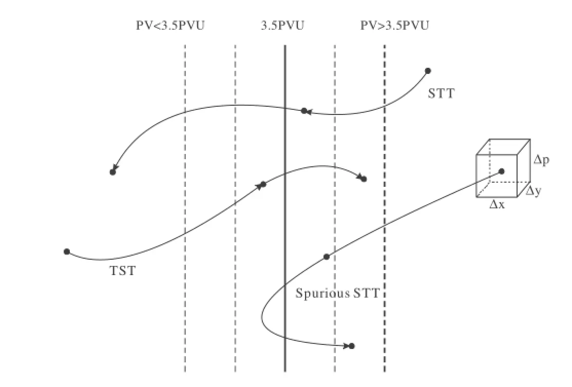
Figure 1.Schematic illustration of the two-way exchange for Lagrangian calculations.

COLs are more frequent during the late spring and summer months， and there are three climatologically preferred regions for COL occurrence: the northern China-Siberia region， the eastern North Pacific， and southern Europe and the eastern Atlantic coast （Nieto et al. 2008）. As a manifestation of Rossby wave breaking， COLs play a vital role in the irreversible mixing between the stratosphere and troposphere in these regions. In Northeast China， cold vortices， which are frequent synoptic systems in spring or summer， often derive from deeply developed COLs. Although precipitation and disastrous weather caused by northeast cold vortices have been widely investigated （Hu， Lu， and Wang 2011； Zhang and Li 2009）， the quantification of STE generated by vortices or COLs in China or East Asia has， to date， been insufficiently studied.

STE in the vicinity of COLs is usually calculated with Eulerian methods， which are based on Eulerian formulations of cross-tropopause fluxes and estimated from each term of the formulations （e.g. Chen， Lü， and Chen 2014； Wei 1987； Wirth 1995； Wirth and Egger 1999）. Compared with the Eulerian methods， trajectory-based Lagrangian computation of the STE is able to identify the source regions， pathways， timescales， etc. of the air parcels involved in the STE procedure， and helps to distinguish the effective exchange（Bourqui 2004； Chen et al. 2010； Fueglistaler， Wernli， and Peter 2004； James et al. 2003； Meloen， Siegmund， and Sigmond 2001； Stohl 1998； Stohl et al. 2003a， 2003b； Vogel et al. 2011）. This study focuses on the COLs in East Asia and aims to quantify the COL-related cross-tropopause exchange.

Methodology

Model and data

In this study， 3D trajectory integrations are performed using the OFFLINE3 diabatic trajectory model， which is a modification of the third edition of the UK Universities Global Atmospheric Modelling Programme Offline Trajectory Code （Methven 1997）. Compared with the regional kinematic trajectory model， the main difference in the diabatic model is the vertical velocity scheme: vertical（cross-isentropic） velocity is expressed with the diabatic heating rate instead of being calculated with the horizontal wind through the continuity equation. By reducing errors in vertical velocity， the diabatic trajectory model can give better results， especially when relatively coarse primary analysis fields are used （Ploeger et al. 2010， 2011）. A comprehensive review of the accuracy of trajectories is given in Methven （1997） and Stohl （1998）.

The OFFLINE3 diabatic trajectory model can be run both forwards and backwards. In this study， trajectories are driven by six-hourly ERA-Interim （European Center for Medium-Range Weather Forecasts Interim Reanalysis）data， and the spatial resolution is T255 （0.75° × 0.75°）（Simmons et al. 2006）. Three-dimensional offline meteorological data， e.g. wind field and temperature， are interpolated to the trajectory locations. At each integration time，values of meteorological fields， including PV， temperature，potential temperature， pressure， and surface pressure are assigned as attributes for the particles moving along the trajectories.

Trajectories are released every 12 h， which is proved sufficient to generate smooth and robust features and overall physical characteristics. The horizontal study domain size is 50° × 50°， moving with COL centers， and the vertical range extends from 700 hPa to 50 hPa， with a vertical resolution of 10 hPa. Each trajectory represents an air mass Δm: Δm = g-1·Δx·Δy·Δp = 6.53 × 1011kg， where the spacing of the air parcel is approximately Δx = Δy = 80 km in the horizontal and Δp = 10 hPa in the vertical. And if the particles cross the tropopause， then the air mass represented by the particles is considered to have crossed the tropopause. The choice of vertical resolution is reasonable in the subtropics but still needs to be verified in the upper troposphere of the tropics where vertical motion is slower.

Definition of the dynamical tropopause

In this study， the PV value of 3.5 PVU （1 PVU = 10-6m2s-1K kg-1）is defined to be the dynamical tropopause. Previous studies have shown that the calculated results of cross-tropopause mass exchange are not very sensitive to the value of PV chosen as the tropopause in the range of 2-5 PVU （Dethof， O'Neill，and Slingo 2000； Pan et al. 2000）. Further study shows that the calculated transports （both upward and downward） decrease as the PV threshold increases from 1.5 to 3.5 PVU， and become relatively constant from 3.5 to 5.5 PVU （Yang and Lü 2003）. In this study， the choice of the dynamical tropopause has been tested by computing the transport cross surface of constantPV values of 2， 2.5， 3， 3.5， and 4 PVU. The results verified the conclusions of Yang and Lü （2003）， showing that 3.5 PVU as the dynamical tropopause may produce slightly weaker cross-tropopause mass fluxes than 2.5 and 3 PVU， but the transport will not increase when the PV values are higher. In the following analysis， 3.5 PVU is defined as the dynamical tropopause and air masses are considered to transmit from the stratosphere to troposphere if their PV value drops from > 3.5 PVU to < 3.5 PVU， and vice versa. Trajectories that cross the 3.5 PVU iso-surface are extended for three days both backwards and forwards. Meanwhile， we introduce residence time τ to eliminate spurious transport. The residence time is a criterion involving the trajectory residing for a period of time longer than a threshold τ on either side of the tropopause before and after having crossed it. And if the condition is not fulfilled， then the transport is considered spurious， as shown in Figure 1.

Selection of COLs

We focus on the COLs lingering over Northeast China in late spring and early summer between 2003 and 2012. First， the COL cases are selected objectively using a similar algorithm as applied in Porcu et al. （2007）， based on the three main characteristics of the COL theoretical model （Nieto et al. 2005）. The algorithm can be summarized as follows:

（1） At 300 hPa， if a grid point is a minimum （within a 10 gpm threshold） in at least six of the eight surrounding grid points， it is identified as a geopotential minimum.

（2） For all the grid points selected in step （1），only those having different wind directions with their adjacent grid points northwards are retained.

（3） Finally， to define the weather system as a COL，the grid points eastward of a candidate COL point should have a thermal front parameter（TFP） higher than that at the COL point.

The first step identifies systems with vortex characteristics and the second step makes sure the vortex is cut off from the westerlies. In the third step， the TFP， defined as in Equation （1）， is the change of temperature （T； units: K）gradient in the direction of its gradient:

TFP serves to verify the baroclinic instability of the system. Further details of the algorithm can be found in Porcu et al. （2007）.

Then， 10 of the candidate COLs with a lifetime longer than five days are chosen subjectively； one COL in each year from 2003 to 2012.

Results and discussion

Air mass fluxes and comparison

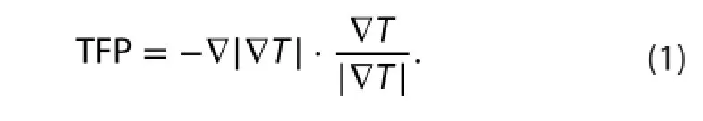
Cross-tropopause fluxes （CTFs） for one COL case in April 2007 are shown as an example. The TST， STT and net fluxes for this case are demonstrated in Figure 2. The TST and STT fluxes were interpolated from the location where they happened to grids， and then the values on the grids were binned every 2° of longitude and latitude. The solid lines in Figure 2 show the 350 hPa geopotential height field at 1800 UTC 29 April 2007 （Figure 2a-c）， 1800 UTC 30 April 2007 （Figure 2d-f）， and 1800 UTC 1 May 2007 （Figure 2g-i）.

On 27 April 2007， the COL started to generate from a deep trough over East Siberia， and cut off on 28 April. Then， the COL intensified and reached maturity on 29 April. Its strength maintained until 1 May and weakened afterwards. As seen in Figure 2b， on 29 April， STT occupied the center， south， and southeast of the COL； this transport spread out to the southwest， south， and southeast on 30 April； and on 1 May， when the COL started to weaken， the STT fluxes curled to the north. TST was mainly in the south and in the east of the trough； and on 1 May， TST increased in the west of the center.

Overall， STT dominated throughout the three days. STT fluxes existed in the center， and in the periphery of the center TST fluxes and STT fluxes were distributed alternately. Net transport in this COL was from the stratosphere to troposphere. For this case， domain-averaged STT and TST fluxes were -1.69 × 10-3and 1.21 × 10-3kg m-2s-1，respectively， the net flux was -0.48 × 10-3kg m-2s-1， and the ratio for TST/STT was 0.716.

Next， we compare our results with previous studies， as listed in Table 1. Sources with asterisks represent studies on global CTFs， and sources without asterisks denote studies on CTFs related with synoptic- or mesoscale weather systems， e.g. extratropical cyclones and streamers. In all of the 10 cases， net CTFs are from the stratosphere to troposphere. The comparison shows that our results are of the same magnitude as results from similar studies on synoptic systems. The CTFs induced by COLs are about one to two orders of magnitude larger than global CTFs. Although STE related with COLs only takes up a fraction of the total STE （Price and Vaughan 1993）， COLs play a significant role in local， rapid air mass exchange.

The preliminary dependencies of the CTFs and total air mass exchange on the intensity of COLs， which is represented by the minimum pressure， are shown in Figure 3. As far as can be revealed by the COL cases used in our study， COLs with STT and TST fluxes （Figure 3a and 3b）generally increase in intensity when minimum pressure decreases， albeit with some exceptions. Similar to the fluxes， the exchanged STT and TST air masses also show a clear dependence on the minimum pressure. Comparedwith the TST fluxes and exchanged mass， the STT fluxes and exchanged mass change more steeply with minimum pressure. These phenomena have also been observed in other studies regarding STE in the vicinity of synoptic systems （Reutter et al. 2015）.

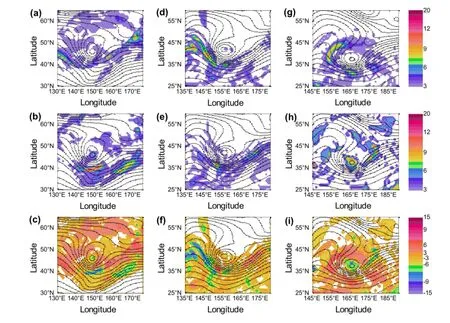
Figure 2.Air mass fluxes for TST （upper row）， STT （middle row）， and net transport fluxes （lower row） on （a-c） 29 April， （d-f） 30 April， and（g-i） 1 May 2007 （units: 10-4kg m-2s-1）. Values on grids were binned every 2° of longitude and latitude. For the net transport， positive values show TST and negative values show STT. Only Absolute values larger than 3 × 10-4kg m-2s-1are shown in the figures.

Table 1.Comparison of mass flux results from previous studies.

Effectiveness of residence time

Residence time is usually used in Lagrangian calculation of STE to eliminate spurious exchange. The results in this study were based on a residence time threshold of 24 h. In order to investigate the sensitivity to residence time， we conducted the above calculations based on residence times of 0， 6， 12，18， and 48 h， and compared the averaged STT and TST fluxes，as shown in Figure 4. The indication is that large numbers of CTFs are associated with time scales smaller than 24 h， and produced reversible exchange. In these cases， 24 h as the residence time threshold helped to exclude spurious exchange and generate reasonable and consistent fluxes. However， the choice of residence time is not unique and it may depend on data resolution， sizes of calculation domains， synoptic systems， etc. A longer residence time would help to focus on more significant exchange.

Summary

In this work， a Lagrangian method for calculating the two-way STE has been applied. COL cases in late spring and early summer over East Asia were selected and the cross-troposphere air mass fluxes in the vicinity of thesecases computed - the aim being to obtain a more accurate understanding of the role that COLs in East Asia play in STE. The diabatic trajectory model used was able to produce more reasonable results because the large-scale motion in large parts of the atmosphere is nearly adiabatic，and the isentropic coordinate system relates better to the physics than the kinematic coordinate system.

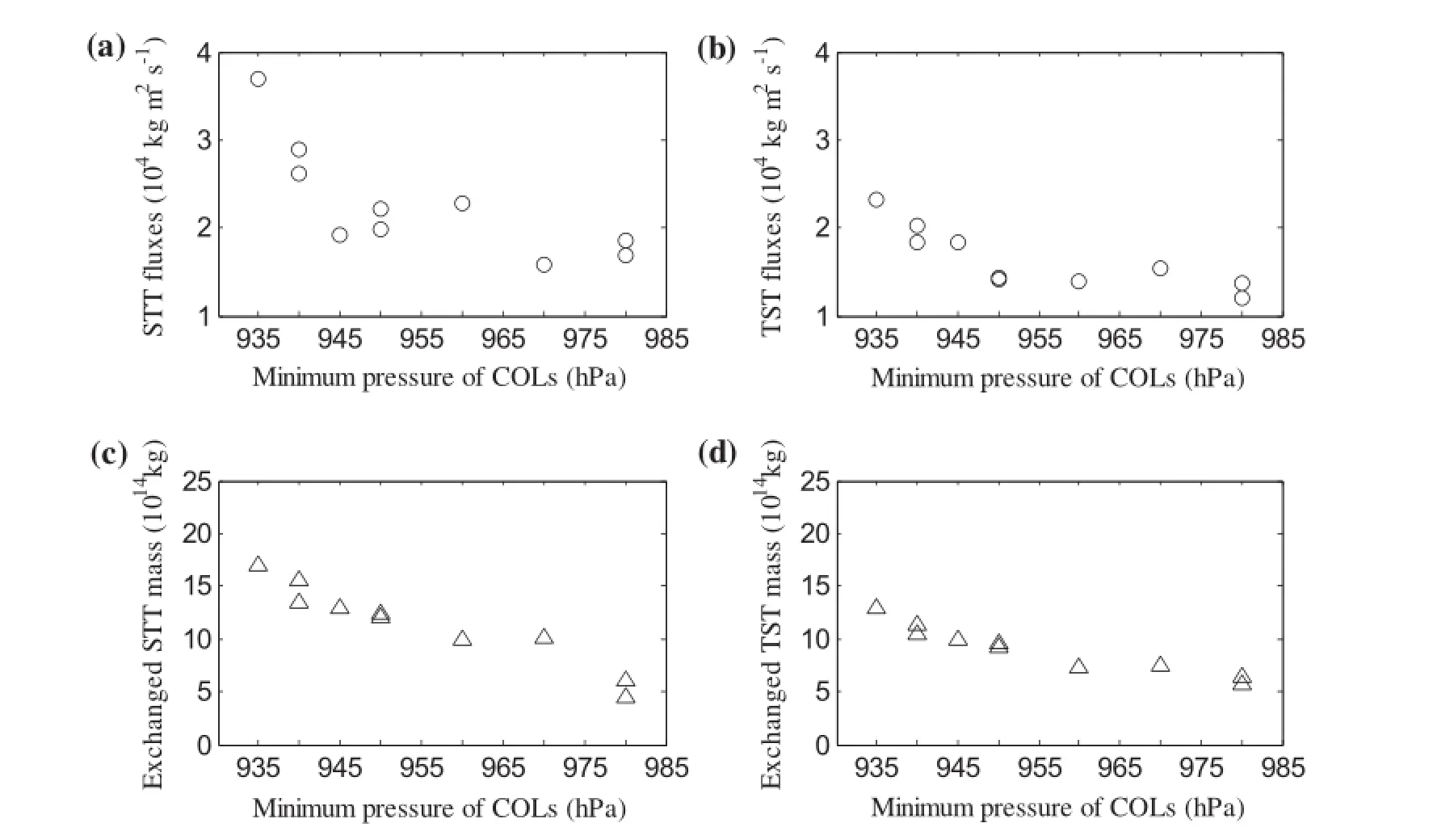
Figure 3.Dependence of the （a， b） CTFs （units: 10-4kg m-2s-1） and （c， d） exchanged mass （units: 1014kg） on the minimum pressure of COLs.

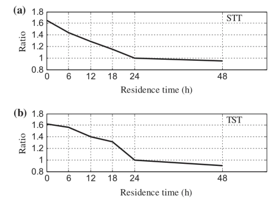
Figure 4.Ratio （results using different residence times/results using 24 h as the residence time） of （a） STT fluxes and （b） TST fluxes.

The results showed that STT dominates the exchange processes in COLs and the net transport is from the stratosphere to troposphere with a magnitude of 10-4kg m-2s-1. The STT and TST fluxes （both with magnitude of 10-3kg m-2s-1） are one to two orders of magnitude larger than global CTFs， and both the STT/TST fluxes and total exchanged air mass during the life cycle of COLs are larger in more intense COLs. The choice of residence time influences the results and， in our study， 24 h was effective in excluding insignificant exchange. COLs contribute to local and efficient air exchange and may favor the rapid transmission of chemicals between the stratosphere and troposphere， although the total exchanged air masses may not be comparable to the total global STE.

Acknowledgements

We thank Dr Sue Yu LIU for providing the OFFLINE3_diab model， and for helpful suggestions. The ERA-interim data were obtained from the European Center for Medium-Range Weather Forecasts， via www.ecmwf.int.

Funding

This work was supported by the Special Fund for Strategic Pilot Technology， Chinese Academy of Sciences ［grant number XDA05040300］.

References

Ancellet， G.， M. Beekmann， and A. Papayannis. 1994. “Impact of a Cutoff Low Development on Downward Transport of Ozone in the Troposphere.” Journal of Geophysical Research 99 （D2）: 3451-3468. doi:10.1029/93jd02551.

Bourqui， M. S. 2004. “Stratosphere-Troposphere Exchange from the Lagrangian Perspective: A Case Study and Method Sensitivities.” Atmospheric Chemistry and Physics 6: 2651-2670.

Chen， B.， X. Xu， J. Bian， X. H. Shi. 2010. “Sources， Pathways and Timescales for the Troposphere to Stratosphere Transport over Asian Monsoon Regions in Boreal Summer.” Chinese Journal of Atmospheric Sciences （in Chinese） 34 （3）: 495-505. Chen， D.， D. R. Lü， and Z. Y. Chen. 2014. “Simulation of the Stratosphere-Troposphere Exchange Process in a Typical Cold Vortex over Northeast China.” Science China Earth Sciences 57（7）: 1452-1463. doi:10.1007/s11430-014-4864-x.

Dethof， A.， A. O'Neill， and J. Slingo. 2000. “Quantification of the Isentropic Mass Transport across the Dynamical Tropopause.”Journal of Geophysical Research 105: 12279-12294. doi:10.1029/2000jd900127.

Ebel， A.， H. Hass， H. J. Jakobs， M. Laube， M. Memmesheimer，A. Oberreuter， H. Geiss， and Y. H. Kuo. 1991. “Simulation of Ozone Intrusion Caused by a Tropopause Fold and Cut-off Low.” Atmospheric Environment. Part a. General Topics 25 （10）: 2131-2144. doi:10.1016/0960-1686（91）90089-p.

Fueglistaler， S.， H. Wernli， and T. Peter. 2004. “Tropical Troposphere-to-Stratosphere Transport Inferred from Trajectory Calculations.” Journal of Geophysical Research 109: D03108. doi:10.1029/2003jd004069.

Hu， K. X.， R. Y. Lu， and D. H. Wang. 2011. “Cold Vortex over North East China and Its Climate Effect.” Chinese Journal of Atmospheric Sciences （in Chinese） 35 （1）: 179-191.

James， P.， A. Stohl， C. Forster， S. Eckhardt， P. Seibert， and A. Frank. 2003. “A 15-Year Climatology of Stratosphere-Troposphere Exchange with a Lagrangian Particle Dispersion Model: 1. Methodology and Validation.” Journal of Geophysical Research 108 （D12）: 8519. doi:10.1029/2002jd002639.

Kentarchos， A. S.， T. D. Davies， and C. S. Zerefos. 1998. “A Low Latitude Stratospheric Intrusion Associated with a Cut-off Low.” Geophysical Research Letters 25 （1）: 67-70. doi:10.1029/97gl03351.

Kentarchos， A. S.， G. J. Roelofs， and J. Lelieveld. 1999.“Model Study of a Stratospheric Intrusion Event at Lower Midlatitudes Associated with the Development of a Cutoff Low.” Journal of Geophysical Research 104 （D1）: 1717-1727. doi:10.1029/1998jd100051.

Lamarque， J. F.， and P. G. Hess. 1994. “Cross-Tropopause Mass Exchange and Potential Vorticity Budget in a Simulated Tropopause Folding.” Journal of the Atmospheric Sciences 51 （15）: 2246-2269. doi:10.1175/1520-0469（1994）051<2246:CTMEAP>2.0.CO；2.

Lü， D. R.， Z. Y. Chen， J. C. Bian， and H. B. Chen. 2008. “Advances in Researches on the Characteristics of Multi-Scale Processes of Interactions between the Stratosphere and the Troposphere and Its Relations with Weather and Climate.” Chinese Journal of Atmospheric Sciences （in Chinese） 32 （4）: 782-792.

Meloen， J.， P. Siegmund， and M. Sigmond. 2001. “A Lagrangian Computation of Stratosphere-Troposphere Exchange in a Tropopause-Folding Event in the Subtropical Southern Hemisphere.” Tellus A 53 （3）: 368-379. doi:10.1034/j.1600-0870.2001.01175.x.

Methven， J. 1997. Offline Trajectories: Calculation and Accuracy，UGAMP， Technical Report 44. Reading， UK: Department of Meteorology， University of Reading.

Nieto， R. L.， L. De Gimeno， P. La Torre， D. Ribera， R. Gallego， J. A. Garcia-Herrera， M. Garcia， A. Nunez， and J. Lorente Redano. 2005. “Climatological Features of Cutoff Low Systems in the Northern Hemisphere.” Journal of Climate 18 （16）: 3085-3103. doi:10.1175/jcli3386.1.

Nieto， R.， M. Sprenger， H. Wernli， R. M. Trigo， and L. Gimeno. 2008. “Identification and Climatology of Cut-off Lows near the Tropopause.” In Trends and Directions in Climate Research，edited by L. Gimeno， R. GarciaHerrera， and R. M. Trigo， Vol. 1146， 256-290. Malden: Wiley-Blackwell.

Pan， L. L.， E. J. Hintsa， E. M. Stone， E. M. Weinstock， and W. J. Randel. 2000. “The Seasonal Cycle of Water Vapor and Saturation Vapor Mixing Ratio in the Extratropical Lowermost Stratosphere.” Journal of Geophysical Research 105: 26519-26530. doi:10.1029/2000jd900401.

Ploeger， F.， P. Konopka， G. Gunther， J. U. Grooss， and R. Muller. 2010. “Impact of the Vertical Velocity Scheme on Modeling Transport in the Tropical Tropopause Layer.” Journal of Geophysical Research 115: D03301. doi:10.1029/2009JD012023.

Ploeger， F.， S. Fueglistaler， J. U. Grooß， G. Gunther， P. Konopka，Y. S. Liu， R. Muller， et al. 2011. “Insight from Ozone and Water Vapour on Transport in the Tropical Tropopause Layer（TTL）.” Atmospheric Chemistry and Physics 11 （1）: 407-419. doi:10.5194/acp-11-407-2011.

Porcu， F.， A. Carrassi， C. M. Medaglia， F. Prodi， and A. Mugnai. 2007.“A Study on Cut-off Low Vertical Structure and Precipitation in the Mediterranean Region.” Meteorology and Atmospheric Physics 96 （1-2）: 121-140. doi:10.1007/s00703-006-0224-5.

Price， J. D.， and G. Vaughan. 1993. “The Potential for Stratosphere-Troposphere Exchange in Cut-off-Low Systems.” Quarterly Journal of the Royal Meteorological Society 119 （510）: 343-365. doi:10.1002/qj.49711951007.

Randel， W. J.， M. Park， L. Emmons， D. Kinnison， P. Bernath， K. A. Walker， C. Boone， and H. Pumphrey. 2010. “Asian Monsoon Transport of Pollution to the Stratosphere.” Science 328（5978）: 611-613. doi:10.1126/science.1182274.

Reutter， P.， B. Škerlak， M. Sprenger， and H. Wernli. 2015.“Stratosphere-Troposphere Exchange （STE） in the Vicinity of North Atlantic Cyclones.” Atmospheric Chemistry and Physics Discussions 15 （2）: 2535-2575. doi:10.5194/acpd-15-2535-2015. Siegmund， P. C.， P. F. J. van Velthoven， and H. Kelder. 1996. “Cross-Tropopause Transport in the Extratropical Northern Winter Hemisphere， Diagnosed from High-Resolution ECMWF Data.”Quarterly Journal of the Royal Meteorological Society 122: 1921-1941. doi:10.1256/smsqj.53608.

Sigmond， M.， J. Meloen， and P. C. Siegmund. 2000. “Stratosphere-Troposphere Exchange in an Extratropical Cyclone， Calculated with a Lagrangian Method.” Annales Geophysicae 18 （5）: 573-582. doi:10.1007/s00585-000-0573-1.

Simmons， A.， S. Uppala， D. Dee， and S. Kobayashi. 2006. “ERAInterim: New ECMWF Reanalysis Products from 1989 Onwards.” ECMWF Newsletter 110: 25-35.

Skerlak， B.， M. Sprenger， and H. Wernli. 2013. “A Global Climatology of Stratosphere-Troposphere Exchange Using the ERA-Interim Dataset from 1979 to 2011.” Atmospheric Chemistry and Physics Discussions 13 （5）: 11537-11595. doi:10.5194/acp-14-913-2014.

Spaete， P.， R. J. Donald， and T. K. Schaack. 1994. “Stratospheric-Tropospheric Mass Exchange during the Presidents' Day Storm.” Monthly Weather Review 122: 424-439. doi:10.1175/1520-0493（1994） 122<0424:SMEDTP>2.0.CO；2.

Sprenger， M.， H. Wernli， and M. Bourqui. 2007. “Stratosphere-Troposphere Exchange and Its Relation to Potential Vorticity Streamers and Cutoffs near the Extratropical Tropopause.”Journal of the Atmospheric Sciences 64 （5）: 1587-1602.doi:10.1175/jas3911.1.

Stohl， A. 1998. “Computation， Accuracy and Applications of Trajectories-A Review and Bibliography.” Atmospheric Environment 32 （6）: 947-966. doi:10.1016/s1352-2310（97）00457-3.

Stohl， A.， P. Bonasoni， P. Cristofanelli， W. Collins， J. Feichter， A. Frank， C. Forster， et al. 2003a. “Stratosphere-Troposphere Exchange: A Review， and What We Have Learned from STACCATO.” Journal of Geophysical Research 108 （D12）: 8516. doi:10.1029/2002jd002490.

Stohl， A.， H. Wernli， P. James， M. Bourqui， C. Forster， M. A. Liniger，P. Seibert， and M. Sprenger. 2003b. “A New Perspective of Stratosphere-Troposphere Exchange.” Bulletin of the American Meteorological Society 84: 1565-1573. doi:10.1175/ bams-84-11-1565.

Vogel， B.， L. L. Pan， P. Konopka， G. Gunther， R. Muller， W. Hall，and T. Campos. 2011. “Transport Pathways and Signatures of Mixing in the Extratropical Tropopause Region Derived from Lagrangian Model Simulations.” Journal of the Atmospheric Sciences 116: D05306. doi:10.1029/2010jd014876.

Wei， M. -Y. 1987. “A New Formulation of the Exchange of Mass and Trace Constituents between the Stratosphere and Troposphere.”Journal of the Atmospheric Sciences 44: 3079-3086. doi:10.1175/1520-0469（1987） 044<3079:ANFOTE>2.0.CO；2.

Wirth， V. 1995. “Comments on “a New Formulation of the Exchange of Mass and Trace Constituents between the Stratosphere and Troposphere”.” Journal of the Atmospheric Sciences 52: 2491-2493. doi:10.1175/1520-0469（1995）052<2491:CONFOT>2.0.CO；2.

Wirth， V.， and J.， Egger. 1999. “Diagnosing Extratropical Synoptic-Scale Stratosphere-Troposphere Exchange: A Case Study.”Quarterly Journal of the Royal Meteorological Society 125: 635-655. doi:10.1256/smsqj.55412.

Yang， J.， and D. R. Lü. 2003. “A Simulation Study of Stratosphere-Troposphere Exchange due to Cut-off-Low over Eastern Asia.”Chinese Journal of Atmospheric Science （in Chinese） 27 （6）: 1031-1044.

Zhang， L. X.， and Z. C. Li. 2009. “A Summary of Research on Cold Vortex over Northeast China.” Climatic Environmental Research （in Chinese） 14 （2）: 218-228.

11 May 2015

CONTACT LÜ Da-Ren ludr@mail.iap.ac.cn

© 2016 The Author（s）. Published by Taylor & Francis

This is an Open Access article distributed under the terms of the Creative Commons Attribution License （http://creativecommons.org/licenses/by/4.0/）， which permits unrestricted use，distribution， and reproduction in any medium， provided the original work is properly cited.