Bo Zeng,Chuan Li,Guo Chen,and Xianjun Long

1.College of Business Planning,Chongqing Technology and Business University,Chongqing 400067,China;

2.School of Management and Economics,University of Electronic Science and Technology,Chengdu 611731,China;

3.Chongqing Key Laboratory of Manufacturing Equipment Mechanism Design and Control,Chongqing 400067,China;

4.School of Electrical&Information Engineering,University of Sydney,Sydney 2006,Australia;

5.College of Mathematics&Statistics,Chongqing Technology and Business University,Chongqing 400067,China

Equivalency and unbiasedness of grey prediction models

Bo Zeng1,2,Chuan Li3,*,Guo Chen4,and Xianjun Long5

1.College of Business Planning,Chongqing Technology and Business University,Chongqing 400067,China;

2.School of Management and Economics,University of Electronic Science and Technology,Chengdu 611731,China;

3.Chongqing Key Laboratory of Manufacturing Equipment Mechanism Design and Control,Chongqing 400067,China;

4.School of Electrical&Information Engineering,University of Sydney,Sydney 2006,Australia;

5.College of Mathematics&Statistics,Chongqing Technology and Business University,Chongqing 400067,China

In order to deeply research the structure discrepancy and modeling mechanism among different grey prediction models,the equivalence and unbiasedness of grey prediction models are analyzed and verifed.The results show that all the grey prediction models that are strictly derived from x(0)(k)+ az(1)(k)=b have the identical model structure and simulation precision.Moreover,the unbiased simulation for the homogeneous exponential sequence can be accomplished.However,the models derived from dx(1)/dt+ax(1)=b are only close to those derived from x(0)(k)+az(1)(k)=b provided that|a|has to satisfy |a|＜0.1;neither could the unbiased simulation for the homogeneous exponential sequence be achieved.The above conclusions are proved and verifed through some theorems and examples.

system modeling,grey prediction models,equivalency and unbiasedness.

1.Introduction

The grey system theory is a useful methodology that focuses on the study of problems involving small samples and poor information[1,2].This methodology deals with uncertain systems using partially known information from which it can generate,exploit and extract useful information[3,4].Therefore,systems’operational behaviors and their laws of evolution can be correctly described and effectively monitored[5].A grey prediction model is one of the most important parts of the grey system theory,and has been employed in many felds,such as industry[6,7], agriculture[8],environment[9],and military[10].In order to solve more practical problems,scientists conducted a lot of researches about the extension and optimization of grey prediction models[11–19],during which dozens of new grey prediction models were established.These models are mainly divided into four types[20,21]as follows:

(i)Type of defnition[2]:GM(1,1,Def)

(ii)Type of whitenization[20]:GM(1,1,Whi)

(iii)Type of extension[21]:GM(1,1,Ext),typically, GM(1,1,x(1)),GM(1,1,x(0)),GM(1,1,b),GM(1,1,Exp), GM(1,1,C);

(iv)Type of discrete[13]:GM(1,1,Dis).

All the above grey prediction models contain only one variable but possess different modeling methods and parameter forms.Although these models have enriched the expressive forms of grey prediction models,at the same time occurrence of inconveniences in choosingan effective model is concerned.In order to solve such an issue,the equivalency and unbiasedness of the above models will be analyzed and studied in this paper.Based on this,models with different forms but the same essence will be categorized then integrated.Eventually,this could reduce the categories of grey prediction models,reduce and even eliminate the low-level repetition during the formation and optimization,and improve the usage effectiveness when grey prediction models are applied.

The rest of this paper is organized as follows.In Section 2,we review some basic knowledge of accumulation generation and some main grey prediction models.The equivalency within grey prediction models are studied in Section 3.In Section 4,we study the unbiasedness of grey prediction models.In Section 5,we verify the theorems proposed and proved in Section 3 and Section 4 through some typical examples.Conclusions are given in Section 6.

2.Accumulated generation operator and grey prediction models

2.1Accumulated generation operator[20]

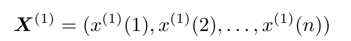
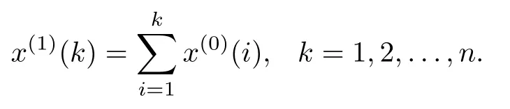
Defnition 1Let X(0)= (x(0)(1),x(0)(2),..., x(0)(n))be an original sequence,x(0)(k)is the value at time k.When the frst-order accumulated generating operator is applied on X(0),we obtain

where

The accumulated generation operator is the foundation of building grey prediction models,and is also a method employed to whitenize a grey process.It plays an extremely important role in grey systems.Through accumulating generation of the sequence,one can potentially uncover a development tendency existing in the process of accumulating grey quantities so that the characteristics and laws of integration hidden in the chaotic original data can be suffciently revealed.For instance,when looking at the fnancial outfows of a family,if we do our computations on a daily basis,we might not see any obvious pattern, however,if our calculations are done on a monthly basis, some pattern of spending,which is somehow related to the monthly income of the family,will possibly emerge.

Accumulating generation of the sequence and its grey exponent law can be seen in Fig.1.

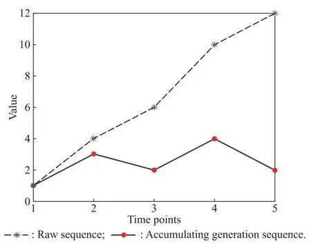
Fig.1 Grey exponent law of accumulating generation sequence

Defnition 2[20] Sequence X(0)and X(1)as stated in Defnition 1,then we obtain a new sequence Z(1)as follows:

where

Then Z(1)is named the mean generation sequence of consecutive neighbors.

2.2GM(1,1,Def)model and GM(1,1,Whi)model

Defnition 3[20] Sequence X(0),X(1)and Z(1)as stated in Defnition 1 and Defnition 2,then

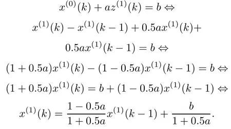
(i)x(0)(k)+az(1)(k)=b is the fundamental form of the GM(1,1)model,called the GM(1,1)of defnition and GM(1,1,Def)for short.

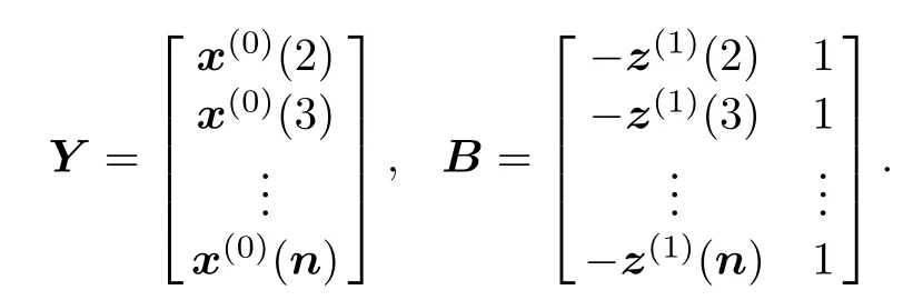
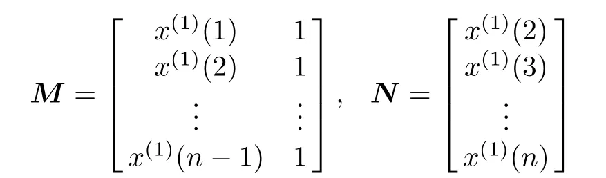
In Defnition 3,ˆa=(BTB)−1BTY,and

2.3GM(1,1,Dis)model[13]

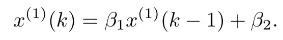
Defnition 4Sequence X(0)and X(1)as stated in Definition 1 and Defnition 2,then

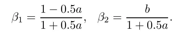
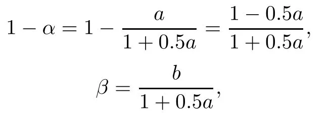
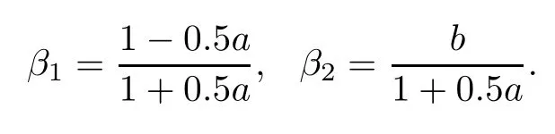
(i)x(1)(k)=β1x(1)(k−1)+β2is called the discrete grey prediction model,or GM(1,1,Dis)model for short.

and

3.Study on equivalency within grey prediction models

In this section,the equivalency within grey models will be analyzed and proved.

Theorem 1Model GM(1,1,Dis)is equal to the GM(1,1,Def),that is,

ProofAccording to Defnition 1 and Defnition 2,

Then

Let

Then

Therefore,

Theorem 2Model GM(1,1,Ext)is equal to the GM(1,1,Dis),that is,

where

ProofAccording to Defnition 1,

Then

Since according to Theorem 1,

Then

NoteThe model GM(1,1,x(1))(that is x(0)(k)= β−αx(1)(k−1))is the representative of the model GM(1,1,Ext),and the proof process of other GM(1,1,Ext) models is the same as Theorem 2,and we will not repeat them now.

Theorem 3[13] When|a|＜ 0.1,the model GM(1,1,Whi)is approximately equivalent to the model GM(1,1,Dis),that is

The proofprocess of Theorem3 can be seen in[13],and omitted here.

According to Theorem 3,the GM(1,1,Dis)model and GM(1,1,Whi)model can be considered as different expressions of the same model.When the value of a is less(that is|a|＜ 0.1),the GM(1,1,Dis)model and GM(1,1,Whi)model can be substituted.

4.Study on unbiasedness of grey prediction models

Defnition 5A grey prediction model,which can simulate homogeneous exponential sequences without error,is called the unbiased grey prediction model,otherwise,the biased grey prediction model.

In this section,we mainly study the unbiasedness of grey prediction models when they are employed in the simulation for the homogeneous exponential sequence.

Theorem 4Model GM(1,1,Def)can simulate the homogeneous exponential sequence without any errors.

ProofLet the sequence X(0)meet the characteristic of homogeneous exponential growth,that is,ˆx(0)(k)=cpk.

According to the GM(1,1,Def)model,we obtain

According to Defnition 1

According to(1)

Put(3)and(4)into(2),we obtain

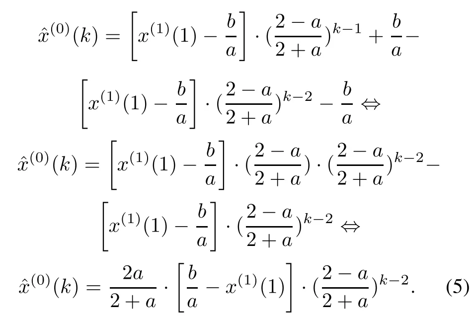
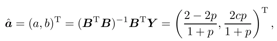
Compute parameters a and b in(5)according to Defnition 3,that is,

Then

and

put it into(5),we obtain

Theorem 5Model GM(1,1,Whi)cannot achieve unbiased simulation for the homogeneous exponential growth sequence.

ProofIt can be known from(2)and Defnition 1,

It can be known from the proof process of Theorem 3 that

then(2)is deformed as follows:

The difference between x(0)(k) = cpkand the GM(1,1,Whi)model is obvious according to(11).Therefore,the model GM(1,1,Whi)cannot achieve the unbiased simulation for the homogeneous exponential growth sequence.The reason is that the parameters a and b of the GM(1,1,Whi)model do not ft by least squares with(6), but come from the GM(1,1,Def)model.Since parameters of one model are established based on another model,the GM(1,1,Whi)model cannot achieve the unbiased homogeneous exponential sequence simulation.

5.Cases

Case 1Verifcation of the grey prediction models’equivalency

Fifteen random numbers generated between 50 and 150 by computer programs are listed in Table 1.

Table 1 Random numbers between 50 and 150

Obviously,data in Table 1 constitute a sequence,that is X(0)= (x(0)(1),x(0)(2),...,x(0)(15))= (104.8, 107.4,...,117.0).The GM(1,1,x(1)),GM(1,1,Def)and GM(1,1,Dis)models of the sequence X(0)are built respectively,and the simulation results of the above three models are presented in Table 2,parameter values of corresponding grey models are as follows:

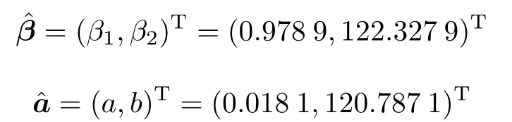
Table 2 Simulation values of GM(1,1,x(1)),GM(1,1,Def)and GM(1,1,Dis)

The two-dimensional scatter plot polygonal line charts of simulation values with the above three models can be seen in Fig.2.

From Table 2 and Fig.2,it is shown that the simulation results of GM(1,1,x(1)),GM(1,1,Def)and GM(1,1,Dis) are identical.Therefore,Theorem 1 and Theorem 2 are verifed.

NoteModel GM(1,1,x(1))is the representative of all GM(1,1,Ext)models in the example.

Case 2Verifcation of simulation results with different models for the homogeneous exponential sequence

Here we construct a sequence X(0)that matches the characteristic of homogeneous exponential growth,which is X(0)(k)=2.5×1.5k(k=1,2,...,15).Now we build the GM(1,1,Whi)and GM(1,1,Dis)models with the sequence X(0)respectively,and the simulation results for the different grey prediction models are shown in Table 3,and the parameter values of corresponding grey models are as follows:

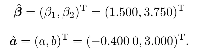
Table 3 Simulation values of GM(1,1,Whi)and GM(1,1,Dis)

Fig.2 Two-dimensional scatter plot polygonal line charts of simulation values

Remark: The two-dimensional scatter plot polygonal line charts of simulation values and residual errors with GM(1,1,Whi) and GM(1,1,Dis)models can be seen in Fig.3.

Fig.3 Raw data,simulation data and residual error with different grey models

It can be seen from Table 3 and Fig.3 that the model GM(1,1,Whi)is not capable of accomplishing the complete simulation for the homogeneous exponential growth sequence(Theorem 4 has been verifed).However,the model GM(1,1,Dis),on the other hand,has the ability (Theorem 3 has been verifed).

Case 3Verifcation of the substitutability between GM(1,1,Dis)and GM(1,1,Whi)when|a|＜0.1

Now we make−a=0.01,0.05,0.10,0.25 and k= 0,1,2,...,9,then four sequences can be obtained by the formula x(0)a(k+1)=e−ak,shown in Table 4.

Establishment of GM(1,1,Whi)and GM(1,1,Dis)models with the sequences Xa=−0.01,Xa=−0.05,Xa=−0.10, Xa=−0.25are conducted here respectively.Then the simulation results for the different grey prediction models are shown in Table 5.

Table 4 Four sequences and their elements

When−a=0.01,0.05,0.10,0.25,the two-dimensional scatter plot polygonal line charts of simulation values and difference between GM(1,1,Whi)and GM(1,1,Dis)can be seen from Fig.4 to Fig.7.

Fig.4 Simulation data and difference between GM(1,1,Whi)and GM(1,1,Dis)(−a=0.01)

Fig.5 Simulation data and difference between GM(1,1,Whi)and GM(1,1,Dis)(−a=0.05)

Fig.6 Simulation data and difference between GM(1,1,Whi)and GM(1,1,Dis)(−a=0.10)

Fig.7 Simulation data and difference between GM(1,1,Whi)and GM(1,1,Dis)(−a=0.25)

From Table 5 and Fig.4–Fig.7,it can be concluded that the simulation results of GM(1,1,Dis)and GM(1,1,Whi) are approximately equivalent when the value of a is less. Moreover,under this circumstance,they can replace each other(Theorem 3 has been verifed).

6.Conclusions

The following conclusions can be drawn according to the above analysis.

(i)According to Theorem 1 and Theorem 2,although GM(1,1,Def),GM(1,1,Ext)(such as GM(1,1,x(1)), GM(1,1,x(0)),GM(1,1,b),GM(1,1,Exp),GM(1,1,C))and GM(1,1,Dis)have different expression forms,they have the identical modeling mechanism.Therefore,substitution between these models is feasible.

(ii)The grey prediction models(or derived models for short)that are strictly derived from the GM(1,1,Def) model are all equivalent to the raw GM(1,1,Def)model, and the unbiased simulation for the homogeneous exponential sequencecan be accomplished.The only difference remains in the expressions of forms and parameters.

(iii)The model GM(1,1,Whi)approximately equals to GM(1,1,Dis)when the grey development coeffcient a is less and satisfes|a|＜0.1.However,the unbiased simulation of the model GM(1,1,Whi)for the homogeneous exponential sequence could not be achieved,due to the fact that the parameters which are used to form GM(1,1,Whi) are borrowed from GM(1,1,Def),instead of being computed by its least squares simulation.

(iv)In order to reduce the repetition status of“identical essence but different form”and improvethe simplicity and employability for grey prediction models,GM(1,1,Dis)is used to represent GM(1,1,Def)and GM(1,1,Ext).This can reduce the number of grey prediction models and avoid the heteromorphism repetition of identical essence models.

(v)According to the above conclusions,grey prediction models are divided into two types,one is GM(1,1,Whi): x(1)(k+1)=(x(1)(k)−b/a)e−ak+b/a,the other is GM(1,1,Dis):x(1)(k)=β1x(1)(k−1)+β2.

[1]A.M.Andrew.Why the world is grey.Grey Systems:Theory and Application,2011,1(2):112–116.

[2]J.L.Deng.The control problem of grey systems.System Control Letter,1982,1(5):288–294.

[3]L.F.Wu,S.F.Liu,L.G.Yao,et al.Grey system model with the fractional order accumulation.Communications in Nonlinear Science and Numerical Simulation,2013,18(7):1775–1785.

[4]Q.X.Li,S.F.Liu,Y.Lin.Grey enterprise input-output analysis.Journal of Computational and Applied Mathematics,2012, 236(7):1862–1875.

[5]S.F.Liu,J.Forrest,Y.J.Yang.A brief introduction to grey systems theory.Grey Systems:Theory and Application,2012, 2(2):89–104.

[6]B.Zeng.Research on electricity demand forecasting based on improved grey prediction model.Journal of Chongqing Normal University(Nature Science),2012,29(6):99–104.

[7]L.C.Hsu.Applying the grey prediction model tothe global integrated circuit industry.Technology and Social Change,2003, 70(6):563–574.

[8]X.W.Ren,Y.Q.Tang,J.Li,et al.A prediction method usinggrey model for cumulative plastic deformation under cyclic loads.Natural Hazards,2012,64(1):1–7.

[9]L.L.Liu,J.Ao,S.Z.Gao.Forecast research into Chinese energy expense based on gray markov chain model.Journal of Chongqing Normal University(Nature Science),2008,25(4): 47–49.

[10]S.G.Cao,Y.B.Liu,Y.P.Wang.A forecasting and forewarning model for methane hazard in working face of coal mine based on LS-SVM.Journal of China University of Mining and Technology,2008,18(2):172–176.(in Chinese)

[11]Z.X.Wang,Y.G.Dang,L.L.Pei.Combinatorial optimization of initial value in GM(1,1)power model.Statistics&Information Forum,2012,27(6):55–58.(in Chinese)

[12]J.Cui.Study on morbidity of NGM(1,1,k)model based on conditions of matrix.Control and Decision,2010,25(7): 1050–1054.(in Chinese)

[13]N.M.Xie,S.F.Liu.Discrete grey forecasting model and its optimization.Applied Mathematical Modeling,2009,33(2): 1173–1186.(in Chinese)

[14]B.Zeng,G.Chen,S.F.Liu.A novel interval grey prediction model considering uncertain information.Journal of the Franklin Institute,2013,350(10):3400–3416.

[15]B.Zeng.Research on prediction modeling method of double heterogeneous data sequence based on core and grey degree. Statistics&Information Forum,2013,28(10):1–6.

[16]H.Jiang,W.W.He.Grey relational grade in local support vector regression for fnancial time series prediction.Expert Systems with Applications,2012,39(3):2256–2262.

[17]Z.Zhao,J.Z.Wang,J.Zhao,et al.Using a grey model optimized by differential evolution algorithm to forecast the per capita annual net income of rural households in China. OMEGA-International Journal of Management Science,2012, 40(5):525–532.

[18]C.I.Chen,H.L.Chen,S.P.Chen.Forecasting of foreign exchange rates of Taiwan’s major trading partners by novel nonlinear grey Bernoulli model NGBM(1,1).Communications in Nonlinear Science and Numerical Simulation,2008,13(6): 1194–1204.

[19]K.Erdal,U.Baris,K.Okyay.Grey system theory-based models in time series prediction.Expert System with Application, 2010,37(2):1784–1789.

[20]S.F.Liu,Y.Lin.Grey systems theory and applications.Berlin Heidelberg:Springer-Verlag,2010:169–190.

[21]X.P.Xiao,S.H.Mao.Methodology for grey prediction and decision-making.Beijing:Science Press,2013:165–200.(in Chinese)

Biographies

Bo Zeng was born in 1975.He received his Ph.D. degree from Nanjing University of Aeronautics and Astronautics of China in 2012.Now he is an associate professor in Chongqing Technology and Business University of China.At present,he is in charge of a project supported by the National Natural Science Foundation of China.His research interest is system prediction,decision-making and evaluation.

E-mail:zbljh2@163.com

Chuan Li was born in 1975.After receiving his Ph.D.degree from Chongqing University of China in 2007,he has been successively a postdoctoral fellow with University of Ottawa,Canada,a research professor with Korea University,South Korea,and a senior research associate with City University of Hong Kong,China.He is currently a professor with Chongqing Technology and Business University,China.His research interests include health maintenances for operational equipments,intelligent system theories and applications.

E-mail:lcctbu@126.com

Guo Chen was born in 1980.He received his Ph.D. degree from the University of Queensland,Australia,in 2010.He is currently a research fellow at the School of Electrical and Information Engineering,the University of Sydney,Australia.He is now conducting research at the Centre for Intelligent Electricity Networks,the University of Newcastle,Australia.From June 2010 to June 2011,he was a research fellow at the Australian National University,Australia.His research interests include complex networks and systems,grey systems theory,optimization and control,intelligent algorithms and their applications in smart grid.

E-mail:guo.chen@sydney.edu.au

Xianjun Long was born in 1980.He received his Ph.D.degree at Sichuan University of China in 2009.He is currently an assistant professor at Chongqing Technology and Business University, China.His research interests include vector optimization,set-valued optimization,vector equilibrium problems and semi-infnite programming problems.

E-mail:xianjunlong@hotmail.com

10.1109/JSEE.2015.00015

Manuscript received March 12,2014.

*Corresponding author.

This work was supported by the National Natural Science Foundation of China(11471059;51375517;71271226),the China Postdoctoral Science Foundation Funded Project(2014M560712),Chongqing Frontier and Applied Basic Research Project(cstc2014jcyjA00024),the Ministry of Education of Humanities and Social Sciences Youth Foundation (14YJAZH033),the Chongqing Municipal Education Scientifc Planning Project(2012-GX-142),and the Higher School Teaching Reform Research Project in Chongqing(1202010).