QIU Xiang (邱翔)

School of Science, Shanghai Institute of Technology, Shanghai 200235, China, E-mail: emqiux@163.com HUANG Yong-xiang (黄永祥), ZHOU Quan (周全)

Shanghai Institute of Applied Mathematics and Mechanics, Shanghai University, Shanghai 200072, China SUN Chao (孙超)

Physics of Fluids Group, University of Twente, AE Enschede, The Netherlands

Scaling of maximum probability density function of velocity increments in turbulent Rayleigh-Bénard convection*

QIU Xiang (邱翔)

School of Science, Shanghai Institute of Technology, Shanghai 200235, China, E-mail: emqiux@163.com HUANG Yong-xiang (黄永祥), ZHOU Quan (周全)

Shanghai Institute of Applied Mathematics and Mechanics, Shanghai University, Shanghai 200072, China SUN Chao (孙超)

Physics of Fluids Group, University of Twente, AE Enschede, The Netherlands

(Received March 31, 2014, Revised May 16, 2014)

In this paper, we apply a scaling analysis of the maximum of the probability density function (pdf) of velocity increments, i.e.,p(τ)=maxp(Δu)～τ-α, for a velocity field of turbulent Rayleigh-Bénard convection obtained at the Taylor-microscalemaxΔuττReynolds numberReλ≈60. The scaling exponentαis comparable with that of the first-order velocity structure function,ζ(1), in which the large-scale effect might be constrained, showing the background fluctuations of the velocity field. It is found that the integral timeT(x/D) scales asT(x/D)～(x/D)-β, with a scaling exponentβ=0.25±0.01, suggesting the large-scale inhomogeneity of the flow. Moreover, the pdf scaling exponentα(x,z) is strongly inhomogeneous in thex(horizontal) direction. The vertical-direction-averaged pdf scaling exponentα~(x) obeys a logarithm law with respect tox, the distance from the cell sidewall, with a scaling exponentξ≈0.22 within the velocity boundary layer andξ≈0.28 near the cell sidewall. In the cell's central region,α(x,z) fluctuates around 0.37, which agrees well withζ(1) obtained in high-Reynolds-number turbulent flows, implying the same intermittent correction. Moreover, the length of the inertial range represented in decade(x) is found to be linearly increasing with the wall distancexwith an exponent 0.65±0.05.

Rayleigh-Bénard convection, scaling, probability density function (pdf)

Introduction

The small-scale fluctuations of turbulent velocity or temperature fields are believed to be universal for high-Reynolds-number turbulent flows[1]This hasbeen recognized as a milestone progress in the turbulence research, known as Kolmogorov 1941 (K41) theory[2]To characterize this universality, theqthorder structure-functions (SFs) are defined as called inertial range, andζ(q)=q/3 for the K41 theory[2]. The above scaling relation has been examined in many different types of turbulent flows by applying the concept of multifractal.[3-6]Besides the SFs analysis, several methodologies have also been proposed, e.g., wavelet-based methods[7-9], Hilbert-based method[10-12], scaling analysis of probability density

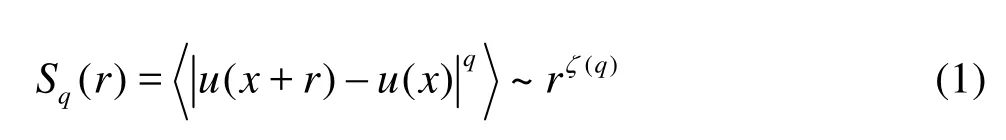
whereris the spatial separation and lies in the so-function (pdf)[13], etc., to quote a few. Note that each method has its own advantages and limitations. For example, due to the nonlocal property of the SFs, it is strongly influenced by large-scale structures, known as infrared (IR) effect, or by energetic structures (e.g., ramp-cliff structure in passive scalar, seasonable forcing in environment data, etc.)[11,14-17], and, however, the wavelet-based (resp. Fourier-based) methods may surfer from higher-order harmonic problem, etc.[11,12,18].

Specifically, for the Rayleigh-Bénard (RB) convection system, buoyant forces are relevant. The flow is then driven by buoyant forces mainly via the so-called thermal plumes[6,19-21]. According to Bolgiano and Obukhov’s arguments, above the so-called Bolgiano length scalelB(see the definition below), instead of the K41 scalingSq(r)～rq/3, the Bolgiano-Obukhov (BO59) scalingSq(r)～r3q/5is expected, at least for the vertical velocity[6,19,20]. Based on the direct spatial velocity measurements using the particle image velocimetry (PIV) technique, Sun et al.[22]found a K41-like scaling with intermittent corrections at the cell, while near the sidewall where thermal plumes abound, vertical velocity (longitudinal direction) and temperature were found to exhibit a different scaling. However, the horizontal velocity is still similar to a K41-like scaling with intermittent corrections, as the influence of the thermal plumes on the horizontal direction is much less than that of the vertical one[22]. For the temperature fluctuations near the cell sidewall, Huang el al.[13]found a K41-like (resp. Kolmogorov-Obukhov-Corrsin, KOC for short) scaling behavior in the probability space, i.e.,pmax(τ)=maxΔθτp(Δθτ)～τ-α, where Δθτ=θ(t+τ)-θ(t) andτis the temporal separation. However, near the cell sidewall where thermal plumes are abundant, the BO59 scaling is expected[6]. They therefore argued that the temperature fluctuations might be considered as a K41-like background fluctuations superposed by thermal plumes (BO59-like structures). For the small-scale statistics in turbulent RB convection, we refer to the reader to the very nice review paper by Lohse and Xia[6].

In this paper, we generalize the idea of pdf scaling to the velocity field measured in a cylindrical turbulent RB convection cell. We first show that the flow is inhomogeneous. It is further found that the integral time scaleThas a power law relation with the wall distancex, i.e.,T～(x/D)-ξ, with a scaling exponentξ=0.25, whereDis the diameter of the cell. Due to the spatial inhomogeneity of the RB flows, we study the pdf scaling in temporal domain. A more than one decade inertial range is observed, which is larger than the one in spatial domain[22]. We find that the scaling exponent (x/D,z) depends onx/D, the distance from the sidewall. A logarithmic law, i.e.(x/D)~γlg10(x/D), with scaling exponentγ=0.22 is found within the velocity boundary layer andγ=0.28 from near the cell sidewall to the cell's central region. Moreover, a power law behavior is found for the length of the inertial range with a scaling exponent 0.69±0.05. Finally, for comparison, the SFs analysis is also performed in temporal domain. Except for the details, the SFs results consist with the pdf scaling results.

1. Scaling behavior of maximum probability density function of velocity increments

More recently, Huang et al.[13]discovered a scaling property of the increment’s pdfs (we work in temporal domain), i.e.,

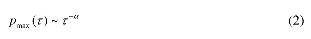
wherepmaxis the maximum value of the pdfpmax=of increments ΔXτ(t)=X(t+τ)-X(t). Hereαis the scaling exponent in probability space and is comparable with the scaling exponent of first-order SFζ(1), at least forH-self-similarity processes.[13]When the pdf scaling approach was applied to the temperature obtained in the near sidewall region of a cylindrical RB convection cell, instead of the BO59 scalingζθ(1)=1/5, a KOC-like scaling beζθ(1)=0.19, a value preferable to the BO59 scaling. It has been shown experimentally that the maximum pdfpmax()τcounts a `real' background fluctuation since the location of thepmax()τis always around ΔXτ≈0[13]. Therefore, the obtained KOC-like scaling havior withθα≈0.33 was obtained[13]. However, the direct estimation of the first-order SF provides has been interpreted as that, at least in the near sidewall region, the temperature fluctuation can be understood as KOC-like background fluctuation superposed with buoyant structures, such as thermal plumes[13].

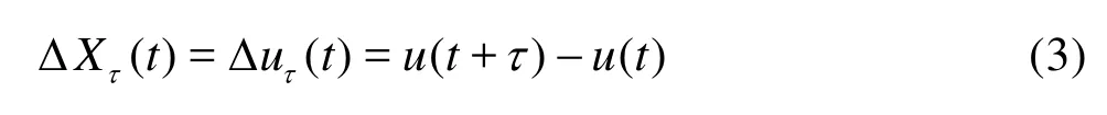
We briefly recall the approach we used in this study. As shown in Huang et al.[13], the pdf scalingpmax()τcan be analytically derived for fractional Brownian motions andH-self-similarity processes in the probability space. Here we obtain the scaling relation Eq.(2) for velocity increments by a dimensional consideration. Taking a turbulent velocity time seriesu(t), the velocity increment is defined as, i.e.,One can define a pdfpτ(ΔXτ) of ΔXτ(t)for a given separation timeτ. Note that the probabilitypτ(ΔXτ) of ΔXτ(t) is a pure number without dimension. Thus one has

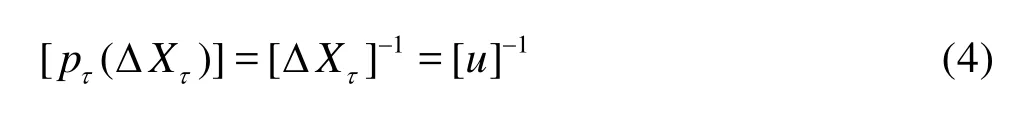
where [·] means dimension. According to Kolmogorov’s similarity hypotheses[1,2], we expect the following power law

whereαis comparable with the first-order SF scaling exponentζ(1) and is to be 1/3 for the Kolmogorov nonintermittent value for homogeneous and isotropic turbulent flows[11,13]. However, the above Eq.(5) may not hold for the whole pdfpτ(ΔXτ). Inspired by a skeleton scaling of pdf found by Huang et al.[10], Huang et al.[13]proposed the maximum pdf maxΔXτ· {pτ(ΔXτ)} at a given scale as a surrogate of the whole pdfpτ(ΔXτ), i.e.,

As was mentioned above, the scaling exponentαis comparable with the first-order SF scaling exponentζ(1)[13]. Experimentally, the maximum pdf of the incrementpτ(ΔXτ) is usually taken around ΔXτ≈0. Therefore, it has been interpreted as background fluctuations of the velocity or temperature fields, in which the effect of large scale structures, e.g., thermal plumes in the RB system, is excluded[13]. More details of the present pdf scaling method can be found in Refs.[11,13].

In this study, we extend the pdf scaling analysis to the horizontal velocity obtained in turbulent RB system by using PIV technique. However, due to the spatial inhomogeneity of the flow (see next section for detail), we consider the approach in the temporal domain. The empirical pdf is estimated as

whereNiis the number of events in theith bin,Nthe total length of the data, anddhthe width of bins. It is found empirically that the pdfpτ(ΔXτ), the maximum pdfpmax()τand the corresponding power law Eq.(6) are almost independent with the range of bin widthdh[13]. Empirically, it is found when the data lengthL≥105(in data points) the error between estimated and given Hurst number is less than 1% see more discussion in Section 2. To ensure a good statistics, we perform in this study a box-counting method to estimate the empirical pdf with data lengthL≥105.

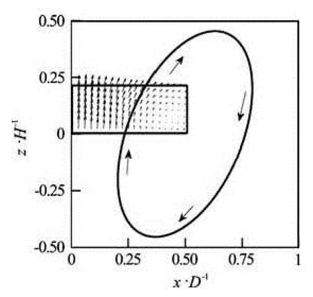
Fig.1 Illustration of the PIV measurement area inx-zplane 0＜x/D＜0.5 and 0＜z/H＜0.21. The time averaged velocity vectorU(x,z) is illustrated by arrows. Note that the flow is inhomogeneous in bothx- andz-directions. The so-called large-scale circulation is illustrated by an ellipse and arrow. The inset shows the cylindrical geometry of the convection cell

2. Experimental data and inhomogeneity of Rayleigh-Bénard flows

2.1Rayleigh-Bénard convection experiment

The convection cell has been described in detail elsewhere[22,23]. Briefly it is a vertical cylinder with top and bottom copper plates and Plexiglas sidewall. The height and the inner diameter of the cell are 0.193 m and 0.19 m, respectively, and thus the aspect ratio isΓ≡D/H≈1. The velocity field was measured by using the particle image velocimetry (PIV) technique. A square-shaped jacket made of flat glass plates and filled with water is fitted round the sidewall, which greatly reduced the distortion effect to the PIV images caused by the curvature of the cylindrical sidewall. The measurements were made from near the cell sidewall to the cell center (see Fig.1). The Prandtl number and Rayleigh number are respectivelyPr≡withgbeing the gravitational acceleration, Δ the temperature difference across the fluid layer, andβ,νandκbeing, respectively, the thermal expansion coefficient, the kinematic viscosity, and the thermal diffusivity of the working fluid (water). The corresponding integral Reynolds numberRe≡WH/ν≈3 600, whereWis the maximal vertical velocity near the sidewall, and the associated Reynolds number based on the Taylor microscale is of the order of60[24]. During the experiment the convection cell was placed inside a thermostat box, which was kept at the mean temperature of the working fluid (40oC), and was tilted by a small angle of ～0.5oso that the velocity measurements were made within the vertical plane of the large-scale circulation (LSC) and at the mid-height of the cell. In each measurement, the measuring region has an area Δx×Δzof 0.00052× 0.00041 m2with a spatial resolution of 0.00066 m, corresponding to 79×63 measured velocity vectors, see Fig.1 and discussion for inhomogeneity below. Polyamid spheres of 50 μm in diameter and 1.03×103kg/m3density were used as seed particles and the laser lightsheet thickness is ～0.0005 m . The measurements lasted 1 h, corresponding to an acquisition time of around 120 turnover times of the large-scale circulation. A total of 7 500 vector maps were acquired with sampling frequency ～2 Hz. Denote the laser-illuminated plane as thexzplane, the horizontal velocity componentu(x,z) and the vertical componentw(x,z) were then obtained. The uncertainty of PIV measurements is about 1%, which is too small to impact the results presented below.

The global Bolgiano length scale, the Kolmogorov length scale and the Taylor microscale are

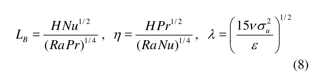
whereHis the height of the cell,Nuthe Nusselt number,uσthe maximum value of theurms, andεthe mean energy dissipation rate, which can be estimated as follows[25]

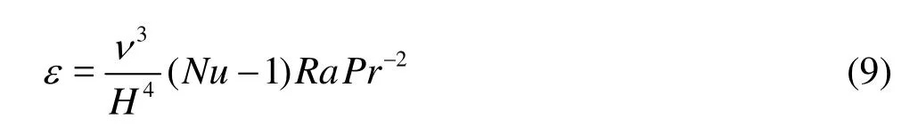
For the present data, we haveLB≈0.005 m, andη≈0.0004 m andλ≈0.008 m[22]. The corresponding global Bolgiano time scale and the Kolmogorov time scale are respectively

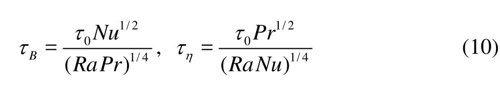
where0τis the turnover time (resp. the period largescale circulation), which is estimated by using the autocorrelation function of the velocity in the near sidewall region. Figure 2 shows the measured autocorrelation function, i.e.,where the first peak corresponds to the turnover time 0τ≈50 s. Therefore, the Bolgiano time scale is aroundτB～1s and the Kolmogrov time scale is aroundτη～0.1s. Hence, the present data does not resolve the Kolmogorov time scale. Note that previous numerical studies have found that energy dissipation rates are spatially inhomogeneous[26-28]. We do not use the Kolmogorov time scaleητto scale the separationτhere due to the lack of measurements of energy dissipation rates. Previously, the horizontal velocity componentu(x,z) has been found to obey the K41-like scaling in spatial domain for both near the sidewall and at the cell center[22]. We note the inertial range in Ref.[22] is quite short. For example, the inertial range in the central region is in the range 0.004 m-0.02 m, around 0.7 decade. We argue here that the spatial inhomogeneous effect, especially in the near sidewall region has taken into account.

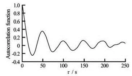
Fig.2 Measured temporal autocorrelation functionρ(x,z,τ) in the near sidewall region. Graphically, the turnover time (resp. the period of the large-scale circulation) is aroundT=50s. The global Bolgiano length scale isLB≈0.005m , the Kolmogorov length scale isη≈0.004 m, and the Taylor’s microscale isλ≈0.008m . The corresponding Bolgiano timescale isτB～1s, and the Kolmogorov time scale isτn～0.1s. Note that both the Bolgiano scale and Kolmogorov scale are inhomogeneous in space

2.2Spatial inhomogeneity of the convection cell

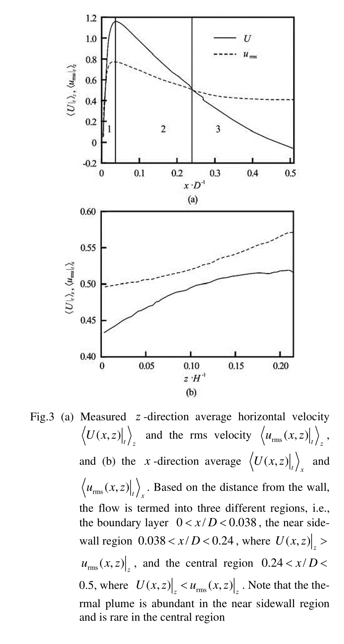
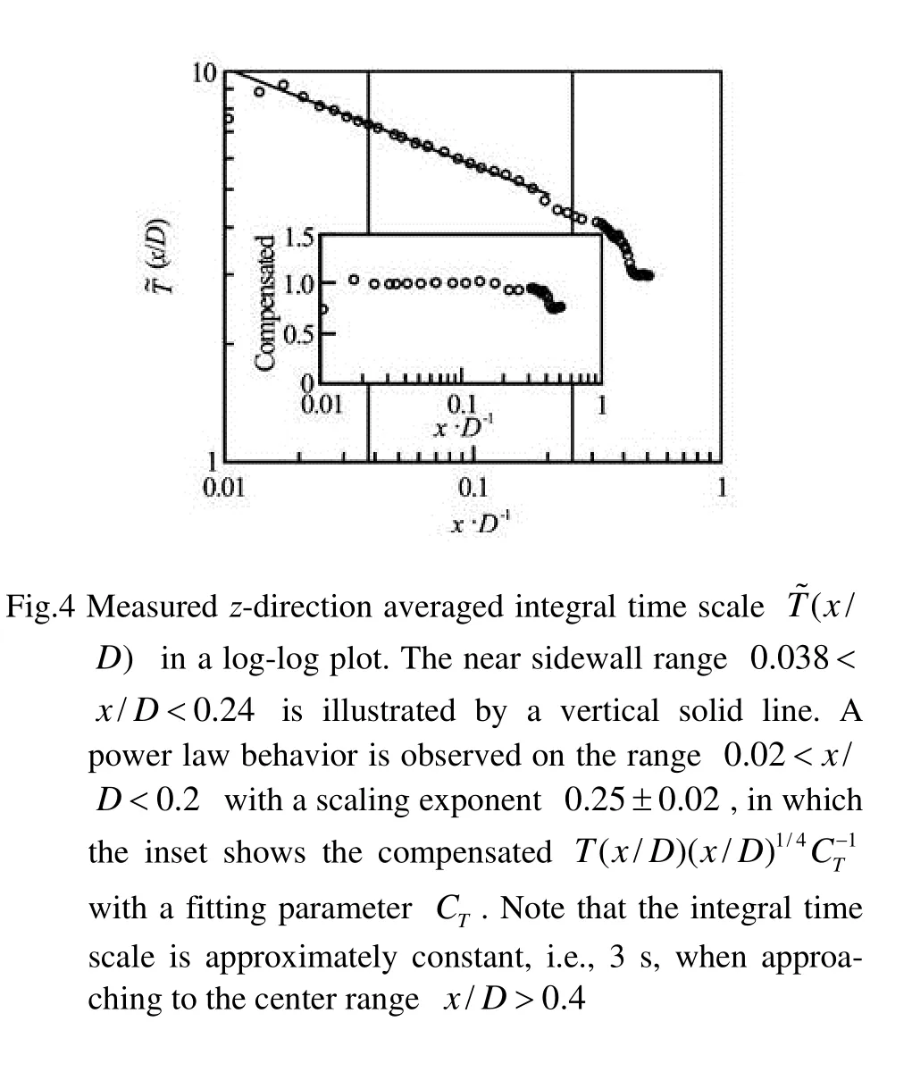
We now turn to the integral time scaleT. The integral time scale is defined as

In practice, the integral time scaleTis calculated on the range 0＜τ＜τz, whereτzis the location of the first zero-crossing. Again, the measuredT(x,z) is a function ofxandz, showing a strongx-direction dependence (not shown here). Figure 4 shows az-direction average integral time scaleT~(x/D) in a loglog plot. A power law behavior is observed on the range 0.02＜x/D＜0.2, i.e.,

whereCT=3.33±0.05 andβ=0.25±0.02 obtained by using a least square fitting algorithm. The integral time scaleTcould be interpreted as average time scale in a statistic sense at a given location. The observed power law indicates that the turbulent structures are decreasing with respect to the wall distancex/D. In the cell centeris a constant, i.e., 3 s when approaching to the cell center. This confirms the validation of the spatial homogeneity in this region[29].

To avoid such inhomogeneous effects and as buoyant forces are exerted on the fluid in the vertical direction, here we consider only the horizontal component of the velocity,u(x,z), in temporal domain.

Figure 5 shows the horizontal velocity componentu(x,z) at several measurement locations. Visually, the velocityu(x,z) is quite stationary in temporal domain at all measurement locations. To relate the scaling behaviors obtained in temporal domain to theoretical predictions in spatial domain, we invoke the elliptic model[32,33], which was advanced based on a systematic second-order Taylor-series expansion of the space-time velocity correlation functionsC(r,)τ. Indeed, several experimental studies in turbulent RB convection have shown that the scaling exponents measured in temporal domain are the same as those obtained in spatial domain if the elliptic model is invoked[30,34,35], and some recentRe-measurements were also based on the elliptic model[36].

3. Results and discussion

3.1Scaling of probability density function

Fig.5 Measured velocityu(x,z) four given locations withz/H≈0.Visually, they are statistical stationary in temporal domain

Fig.6 Measured pdfp(Δuτ) foru(x,z) at locationx/D≈0.42 andz/H≈0.20 ith 5×5 velocity grids and a time separationτ=10s, in which the normal distribution is illustrated by a solid line. The inset shows the integral kernelp(Δuτ)Δuτfor the first-order structure-function. The location of maximum pdf (illustrated by a vertical line) is around Δuτ≈0, indicating thatpmax(τ) almost has no contribution to the first-order structure-function. The pdf scaling ofpmax(τ) thus represents a background fluctuation without the influence of large scale structures, e.g., thermal plumes, large-scale-circulation, etc.

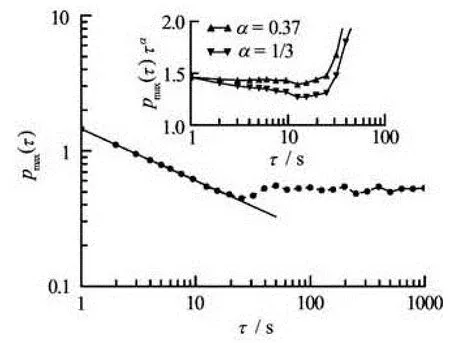
Fig.7 Measuredpmax(τ) for the horizontal velocityu(x,z) at locationx/D=0.42 andz/H=0.20 with 10×10 velocity grids. A more than one decade inertial range is observed on the range 1s≤τ≤20s with a scaling exponentα≈0.37, a scaling exponent reported for the turbulent velocity of high-Reynolds homogeneous and isotropic turbulent flows. The inset shows the compensatedpmax(τ)ταrespectively withα=1/3 (downtriangles) andα=0.37 (triangles) to emphasize the power law behavior

Figure 6 shows the empirical pdfpτ(Δuτ), foru(x,z) at the locationx/D≈0.42 andz/H≈0.20 with 5×5 velocity grids and a time separationτ=10 s, in which the normal distribution is illustrated by a solid line. The correspondingρmax()τis illustrated by a vertical solid line. Note that the location of the maximum pdf maxΔuτpτ(Δuτ) is around Δuτ≈0 for all separation scales. To compare with the first-order SF, we show the integral kerneluτpτ(Δuτ) as inset. Note that theρmax()τalmost has no contribution to the SF[13]. Therefore, the pdf scaling represents a real background fluctuation without the influence of largescale structures, e.g., thermal plumes, LSC etc.. Figure 7 showsρmax()τmeasured atx/D=0.42 andz/H=0.42, the position close to the cell's central region. To acquire accurate statistics,ρmax()τwas calculated within an area of 0.000066×0.000066 m2, i.e., 10×10 velocity vectors, corresponding to 6.4×105(10×10× 7 500×0.85, number of velocity vectors inx-direction × number of velocity vectors inz-direction × number of vector maps × mean ratio of valid velocity vectors) data points. According to Ref.[13], this can provide a quite good estimation ofαif there exists any powerlaw behavior. The inset shows the compensatedρmax(τ)τ-αwithα=1/3 andα=0.37. Visually, a quite clean power-law behavior is observed for the range 1s≤τ≤20s with a scaling exponentα≈0.37. It is interesting to note that the index value ofαhere is consistent with the first-order SF scaling exponent,ζ(1)=0.37, reported in other studies for high-Reynolds-number turbulent flows[3,4,37]. This confirms the pdf scaling for the horizontal velocity and implies, despite of a relatively small Reynolds number, the same intermittent correction as those in high-Reynolds-number turbulent flows.α(x,z),ρmax(τ) at each position (x,z) was calcu-

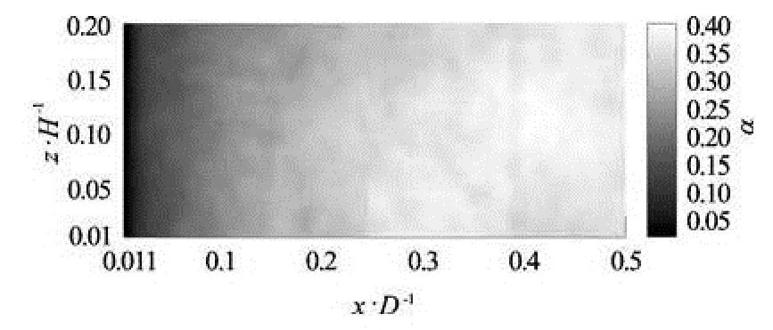
Fig.8 Measuredα(x,z) of the horizontal velocity on the measurement domain 0.01＜x/D＜0.5 and 0.01＜z/H＜0.21 with a 5×5 spatial velocity grids and 1 moving grid5in bothxandzdirections. It corresponds to 1.6×10 data points for each realization. Visually, the measuredα(x,z) shows a strongx-dependence

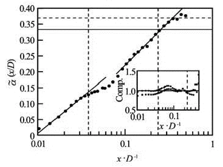
Fig.9 Thez-direction spatial averaged scaling exponents(x/D) in a semilog plot. The index values 1/3 and 0.37 are illustrated respectively by the horizontal solid line and dashed line. The vertical dashed line indicates the range of the velocity boundary layer,x/D＜0.038, the near sidewall range 0.038＜x/D＜0.24 and the central region 0.24＜x/D, respectively. Logarithm laws are observed in the range 0.01＜x/D＜0.03 and 0.1＜x/D＜0.4 respectively with scaling exponents 0.22±0.02 and 0.28±0.02. The inset shows the compensated curves to emphasize the observed log laws

To further evaluate the spatial distribution of lated within an area of 5×5 velocity vectors, corresponding to 5257 5000.85=1.6 10××× (number of velocity vectors × number of vector maps × mean ratio of valid velocity vectors) data points, which is long enough to provide a good estimation ofα[13]. We plot the spatial distribution of the estimatedα(x,z) in Fig.8, which shows a strongx-dependence. It implies the inhomogeneity in probability space and might be understood as the effect of the sidewall (resp. thermal plumes). On the other hand, thez-dependence ofα(x,z) is much weaker. We thus calculate thezaveraged (vertical-direction-averaged) exponentα(x) as

where Δz=0.041m≈0.2H. Figure 9 shows the measured(x) in a semilog plot, in which the index values 1/3 and 0.37 are illustrated respectively by horizontal solid and dashed lines. Graphically,(x) reaches the K41 value 1/3 aroundx/D=0.26, and arrives 0.37 aroundx/D=0.32. This further confirms previous findings that in the central region of the cell the velocity field exhibit the same scaling behavior that one would find in homogeneous and isotropic Navier-Stokes turbulence[22,29,30,38]. Moreover, two logarithm laws are observed in the velocity boundary layer 0.01＜x/D＜0.03 and 0.1＜x/D＜0.44 i.e.,

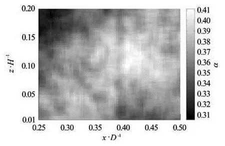
Fig.10 Re-plot measuredα(x,z) in the measurement domains 0.25＜x/D＜0.5 and 0.01＜z/H＜0.21 with a 5×5 spatial velocity grids and 1 moving velocity grid in both directions. A spatial pattern, fluctuating over the range 0.28＜α＜0.41, is observed, indicating an inhomogeneous property of the RB convection system even in the cell center

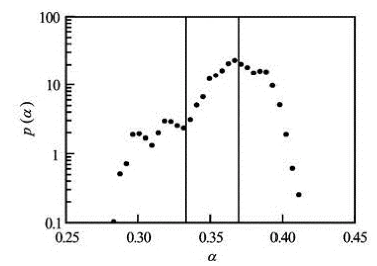
Fig.11 Empirical probability density function ofαon the range 0.25＜x/D＜0.5. The vertical line indicates the valueα=1/3 andα=0.37. Note that the most probability value is around 0.37

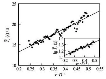
Fig.12 Thez-direction averaged length of the power law range(x/D) in linear-linear plot, in which the solid line is a linear fitting with a slopeφ=28.6±1.9. The inset shows the time length of the measured(x/D) in decades, in which the solid line is a least square fitting with a slope 0.69±0.05. Note that the measured(x/D) strongly depends on the wall distancex/D

We denote hereTIas the time length of the inertial range forpmax()τ, i.e.,

whereSτis the lower end of the inertial range, i.e., 1 s, andEτis the end of the inertial range. The measuredTIis showingx-dependent (not shown here). Note that in the present case, we do not have the resolution of the Kolmogrov scale, which is in the order –0.1 s. Therefore, if we take the 1 s as the lower endSτof the inertial range, then the corresponding length of the inertial range is at least 1.0-1.4 decades in the logarithm frame, i.e.,TI=lg10(τE)-lg10(τS). This inertial to be 0.004 m＜r＜0.02 m , corresponding to 0.7 decade, in spatial domain in the central region of the cell. The reason for the different length of the inertial range in the spatial and temporal domains might be the effect of the spatial inhomogeneity of the turbulent flow range is significant larger than the one reported in Ref.[22], in which an inertial range is typically foundin RB cell as we emphasized previously, see Figs.3 and 10. Figure 12 displays thez-direction averaged(x/D), in which the inset shows the corresponding length in decades(x/D). Graphically, it suggests a linear relation

with the slopeφ=28.6±1.9. For the measuredTI, a linear relation is found to be, i.e.,

with the slopeφ=0.69±0.05. We understand these wall-dependent relations as the effect of both wall boundary and thermal plumes, which is also associated with the near sidewall region.

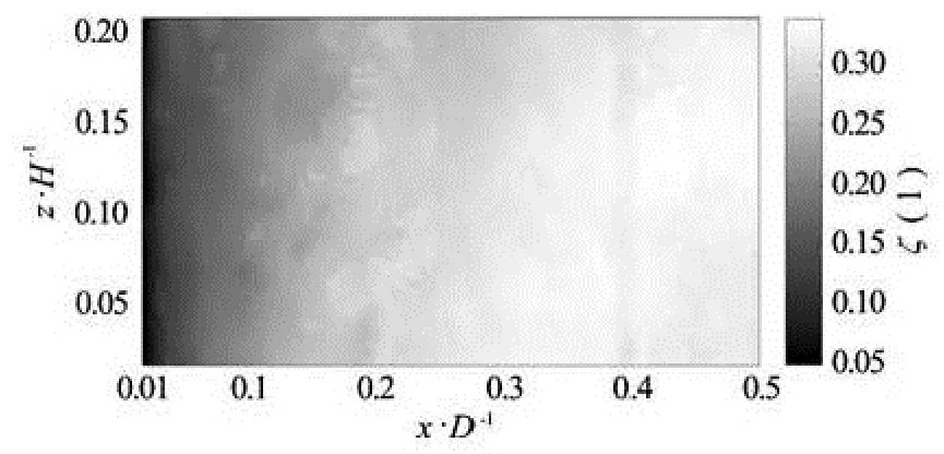
Fig.13 Measured first-order SF scaling exponentζ(1,x,z) by using the same moving-grid algorithm for the pdf scaling. Note that the measuredζ(1,x,z) also showsx-dependence

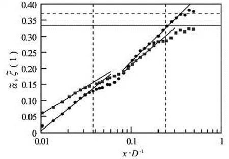
Fig.14 Thez-direction averagedξ(1,x) (squares) in a semilog plot, in which the index values 1/3 (solid line) and 0.37 (dashed line) are also shown. The vertical dashed line indicates the range of the velocity boundary layer,x/D＜0.038, the near sidewall range 0.038＜x/D＜0.24 and the central region 0.24＜x/D, respectively. Logarithm law is observed in the velocity boundary layer with a scaling exponent 0.17±0.22 and on the range 0.1＜x/D＜0.2 with a scaling exponent 0.24±0.02, respectively. For comparison, the measuredα~ is also reploted (circles)

3.2First-order structure function: A comparison

For comparison, we perform the same algorithm for the first-order SF in temporal domain. Figure 13 shows the measured scaling exponentζ(1,x,z) for the first-order SF. Graphically, it is alsox-dependent, especially on the near sidewall region. This is consistent with Fig.8. The fluctuation range of the scaling exponentαis larger thanζ(1). Figure 14 shows thez-direction averaged, in which the solid line is the logarithm fitting respectively with scaling exponent 0.17±0.02 and 0.24±0.02. It is close to the K41 value whenx/D＞0.2. We could term the measuredinto two regimes. The first regime is on the range 0.01＜x/D＜0.1, whereThe second one isx/D＞0.1, in whichFigure 15 reproduces the measuredζ(1,x,z) in the range0.25＜x＜0.5. Visually, it seems that, despite of a small value, the measuredζ(1) is a smooth version ofα. However, both the first-order SF scalingζ(1) and the pdf scalingαshow a similar spatial pattern and wall dependence.

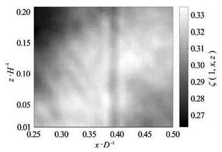
Fig.15 Replot the measuredζ(1,x,z) in the range 0.25＜x/D＜0.5, which fluctuates in the range of 0.26＜ζ(1)＜0.33. A similar spatial pattern as shown in Fig.10 is observed. Note that the pattern provided by SF can be seen as a smooth version of the one provided by the pdf

3.3He’s Elliptic model

As we mentioned above that to convert the temporal domain to spatial domain, Taylor’s frozen hypothesis is usually applied[2]. However, in RB cell, conditions for Taylor’s hypothesis are not satisfied[39]. Note that Taylor’s frozen hypothesis is the first-order expansion of the correlation function in which only the mean convection velocity is involved[32]. More recently, He and Zhang[32]proposed a second-order expansion theory to convert the measurement from the temporal domain to spatial domain. This second-order formula is named as elliptic model, i.e.,

Fig.16 A statistics test of the length dependentα(N) andζ(1,N) (circles) for the Hurst numberH=1/3 with 1 000 realizations for each fBm simulation with variousNin data points. (a) The measured scaling exponentsα(N) (circles) andζ(1,N) (squares). The error bar is the standard deviation of the measured scaling exponent from the 1 000 realizations. The solid line is a power law fitting of the error bar. (b) The corresponding errorbar (closed symbols) and relative errorEr(N)=[H-ζ(1,N)]/H(open symbols). The solid line is the power law fitting with scaling an exponent 0.50±0.02 for the measured errorbar and the relative error for the first-order SF, and an scaling exponent 0.91±0.02 for the relative error for the pdf scaling, respectively. Note that whenN＞105, the first-order SF provides a relative error less than 0.1% and a standard deviation less than 3%. The vertical dashed line indicates the validation data length from PIV measurement

in whichU0is a characteristic convection velocity proportional to the mean velocityU, andVis the sweeping velocity associated with the rms. velocity and the shear-induced velocity[32]. The validation of He’s model in RB cell has been verified experimentally in several works[34,36,40]. However, Zhou et al.[40]found that the convection velocityU0and sweeping velocityVare indeed have spatial distribution. It is not easy to relate our temporal scaling exponentsζ(1) andαwith the spatial domain ones since the flow here is spatial inhomogeneous. Therefore, one cannot perform one to one comparison between the present results with the ones reported in Ref.[22].

3.4Finite size effect of data sample

To exclude the effect of finite sample size, we perform a fractional Brownian motion (fBm) simulation with a Hurst numberH=1/3. fBm simulation was realized by using a Wood-Chan algorithm[41]with 1 000 realizations and various data lengthN. We chose the data length 104＜N＜3.2× 106. The scaling exponent of the first-order SFζ(1,N) is then estimated on the range 10＜τ＜1000 data points. Figure 16 shows the measuredζ(1,N), in which the errorbar was the standard deviation of the estimatedζ(1,N) from 1 000 realizations. The solid line is power law fitting of the error-bar. Note that the estimatedζ(1,N) is asymptotic to the givenHvery quickly. The inset shows an relative of the estimatedζ(1,N), i.e.,Er(N)=[H-ζ(1,N)]/H(circles), andδζ(1,N)/H(squares), respectively. The solid lines are power law fitting with slope 0.50±0.02 for the error-bars and the relative error for the first-order SF, and 0.09± 0.02 for the relative error of pdf scaling, respectively. The former slope 0.5 is consistent with the previously finding for the pdf scaling[13]. Note that whenN＞105, the first-order SF provides a relative error less than 0.1% and a standard deviation less than 3%. In the present study, the data length is about 1.6×105, which provides a quite good statistical convergence for both the first-order SF and the pdf scaling. Therefore, the experimental results reported here cannot be the finite size sample effect.

4. Conclusions

In summary, in this study, we have extended our previous work[13]and generalized the pdf scaling analysis to turbulent velocity in turbulent RB convection cell. The integral time scale is found to obey a power law in the range 0.02＜x/D＜0.2 with a scaling exponent 0.25±0.02. We confirmed the pdf scaling for the horizontal velocity in probability space. The estimatedα(x,z) is strongly inhomogeneous with respect to thex-direction and thez-dependence ofα(x,z) is much weaker, which can be understood as the effect of the sidewall. The scaling exponentα(x,z) shows its own spatial pattern. Moreover, thez-direction-averagedα~(x) obeys a logarithm law with respect tox, the distance from the sidewall, with a sca-ling exponent =0.220.02β± in the velocity boundary layer, i.e.,x/D＜0.03, andβ=0.28±0.02 on the range 0.1＜x/D＜0.4, respectively. In the cell’s central region, theα(x,z) fluctuates around 0.37. Despite of the quite low Reynolds number here, the scaling exponentα=0.36±0.02 is consistent with the first-order SFs scaling exponentζ(1) for high-Reynolds-number turbulent flows reported in other studies. It is interesting to note that the pdf itself has almost the same intermittent correction as the firstorder SFs scaling in high-Reynolds-number turbulent flows. Furthermore, thez-direction averaged length of the inertial rangeis increasing linearly with the distance from the wall. Equivalently, the measured length of the inertial range represented in decadeis linear increasing withx/Dwith a slope 0.69±0.05. Finally, the pdf scaling analysis is compared with the first-order SF. The experimental results show similar spatial pattern for bothαandζ(1), and also similar wall-dependence ofz-direction averaged. Note that the numerical difference between the measuredαandζ(1) is from the fact that the pdf scaling reflect the background fluctuations, while the first-order SF takes all the turbulent structures into account, including the thermal plumes, LSC, etc..

[1] KOLMOGOROV A. N. Local structure of turbulence in an incompressible fluid at very high Reynolds numbers[J].Doklady Akademii Nauk SSSR,1941, 30(4): 301-305.

[2] FRISCH U.Turbulence: The legacy of AN Kolmogorov[M]. Cambridge, UK: Cambridge University Press, 1995.

[3] SHE Z. S., LEVEQUE E. Universal scaling laws in fully developed turbulence[J].Physical Review Letter,1994, 72(3): 336-339.

[4] ARNEODO A., BAUDET C. and BENZI R. et al. Structure functions in turbulence, in various flow configurations, at Reynolds number between 30 and 5000, using extended self-similarity[J].Europhysics Letters,1996, 34(6): 411-416.

[5] SREENIVASAN K., ANTONIA R. The phenomenology of small-scale turbulence[J].Annual Review Fluid Mechanics,1997, 39: 435-472.

[6] LOHSE D., XIA K. Q. Small-scale properties of turbulent Rayleigh-Benard convection[J].Annual Review Fluid Mechanics,2010, 42: 335-364.

[7] LASHERMES B., ROUX S. and ABRY P. Comprehensive multifractal analysis of turbulent velocity using the wavelet leaders[J].European Physical Journal B,2008, 61(2): 201-215.

[8] KOWAL G., LAZARIAN A. Velocity field of compressible magnetohydrodynamic turbulence: Wavelet decomposition and mode scalings[J].Astrophysics Jour-nal,2010, 720: 742-756.

[9] LORD J. W., RAST M. P. and MCKINLAY C. et al. Wavelet decomposition of forced turbulence: Applicability of the iterative Donoho-Johnstone threshold[J].Physics of Fluids,2012, 24(2): 025102.

[10] HUANG Y. X., SCHMITT F. G. and LU Z. M. et al., An amplitude-frequency study of turbulent scaling intermittency using Hilbert spectral analysis[J].Europhysics Letters,2008, 84(4): 40010.

[11] HUANG Y. X. Arbitrary-order hilbert spectral analysis: Definition and application to fully developed turbulence and environmental time series[D]. Doctoral Thesis, Lille, France: University des Sciences et Technologies de Lille and Shanghai, China: Shanghai University, 2009.

[12] HUANG Y. X., SCHMITT F. G. and HERMAND J. P. et al. Arbitrary-order Hilbert spectral analysis for time series possessing scaling statistics: Comparison study with detrended fluctuation analysis and wavelet leaders[J].Physical Review E,2011, 84(1): 016208.

[13] HUANG Y. X., SCHMITT F. G. and ZHOU Q. et al., Scaling of maximum probability density functions of velocity and temperature increments in turbulent systems[J].Physical of Fluids,2011, 23(12): 125101.

[14] DAVIDSON P. A., PEARSON B. R. Identifying turbulent energy distribution in real, rather than fourier, space[J].Physical Review Letters,2005, 95(21): 214501.

[15] HUANG Y. X., SCHMITT F. G. and LU Z. M. et al., Analysis of daily river flow fluctuations using empirical mode decomposition and arbitrary order Hilbert spectral analysis[J].Journal of Hydrology,2009, 373(1-2): 103-111.

[16] HUANG Y. X., SCHMITT F. G. and LU Z. M. et al.. Second-order structure function in fully developed turbulence[J].Physical Review E,2010, 82(2): 26319.

[17] HUANG Y. X., BIFERALE L. and CALZAVARINI E. et al. Lagrangian single particle turbulent statistics through the Hilbert-Huang transforms[J].Physical Review E,2013, 87(4): 041003.

[18] HUANG N. E., SHEN Z. and LONG S. R. A new view of nonlinear water waves: The hilbert spectrum[J].Annual Review of Fluid Mechanics,1999, 31: 417-457.

[19] BOLGIANO R. Turbulent spectra in a stably stratified atmosphere[J].Journal of Geophysical Research,1959, 64(12): 2226-2229.

[20] OBUKHOV A. M. On the influence of archimedean forces on the structure of the temperature led in a turbulent flow[J].Doklady Akademii Nauk SSSR,1959, 125: 1246-1248.

[21] AHLERS G., GROSSMANN S. and LOHSE D. Heat transfer and large scale dynamics in turbulent Rayleigh-Benard convection[J].Review of Modern Physics,2009, 81(2): 503-537.

[22] SUN C., ZHOU Q. and XIA K. Q. Cascades of velocity and temperature fluctuations in buoyancy-driven turbulence[J].Physical Review Letters,2006, 97(14): 144504.

[23] ZHOU Q., SUN C. and XIA K. Q. Experimental investigation of homogeneity, isotropy, and circulation of the velocity field in buoyancy-driven turbulence[J].Journal of Fluid Mechanics,2008, 598: 361-372.

[24] GASTEUIL Y., SHEW W. and GILBERT M. et al., Lagrangian temperature, velocity, and local heat flux measurement in Rayleigh-Benard convection[J].Physical Review Letters,2007, 99(23): 234302.

[25] GROSSMANN S., LOHSE D. Fluctuations in turbulent Rayleigh-Benard convection: The role of plumes[J].Physics of Fluids,2004, 16(12): 4462-4472.

[26] BENZI R., TOSCHI F. and TRIPICCIONE R. On the heat transfer in Rayleigh-Benard systems[J].Journal of Statistical Physics,1998, 93(8): 901-918.

[27] CALZAVARINI E., TOSCHI F. and TRIPICCIONE R. Evidences of bolgiano-obhukhov scaling in three-dimensional Rayleigh-Benard convection[J].Physical Review E,2002, 66(1): 016304.

[28] KUNNEN R., CLERCX H. and GEURTS B. et al. Numerical and experimental investigation of structure-function scaling in turbulent Rayleigh-Benard convection[J]. Physical Review E,2008, 77(1): 016302.

[29] ZHOU Q., XIA K. Q. Comparative experimental study of local mixing of active and passive scalars in turbulent thermal convection[J].Physical Review E,2008, 77(5): 056312.

[30] ZHOU Q., XIA K. Q. Disentangle plume-induced anisotropy in the velocity field in buoyancy-driven turbulence[J].Journal of Fluid Mechanics,2011, 684: 192-203.

[31] ZHOU Q., XIA K. Q. Measured instantaneous viscous boundary layer in turbulent Rayleigh-Benard convection[J].Physical Review Letters,2010, 104(10): 104301.

[32] HE G. W., ZHANG J. B. Elliptic model for space-time correlations in turbulent shear flows[J].Physical Review E,2006, 73(5): 055303(R).

[33] ZHAO X., HE G. W. Space-time correlations of fluctuating velocities in turbulent shear flows[J].Physical Review E,2009, 79(2): 046316.

[34] HE X. Z., HE G. W. and TONG P. Small-scale turbulent fluctuations beyond Taylor’s frozen-flow hypothesis[J].Physical Review E,2010, 81(6-2): 065303(R).

[35] HE X. Z., TONG P. Kraichnan’s random sweeping hypothesis in homogeneous turbulent convection[J].Physical Review E,2011, 83(3-2): 037302.

[36] HE X. Z., FUNFSCHILLING D. and NOBACH H. et al. Transition to the ultimate state of turbulent Rayleigh-Benard convection[J].Physical Review Letters,2012, 108(2): 024502.

[37] BENZI R., CILIBERTO S. and TRIPICCIONE R. et al. Extended self-similarity in turbulent flows[J].Physical Review E,1993, 48(1): 29-32.

[38] NI R., HUANG S. D. and XIA K. Q. Local energy dissipation rate balances local heat flux in the center of turbulent thermal convection[J].Physical Review Letters,2011, 107(17): 174503.

[39] SHANG X. D., XIA K. Q. Scaling of the velocity power spectra in turbulent thermal convection[J].Physical Review E,2001, 64(6): 065301.

[40] ZHOU Q., LI C. M. and LU Z. M. et al. Experimental investigation of longitudinal space-time correlations of the velocity field in turbulent Rayleigh-Benard convection[J].Journal of Fluid Mechanics,2011, 683: 94-111.

[41] WOOD A., CHAN G. Simulation of stationary Gaussian processes in [0, 1] d[J].Journal of Computational and Graphical Statistics,1994, 3(4): 409-432.

10.1016/S1001-6058(14)60040-8

* Project supported by the Natural Science Foundation of China (Grant Nos. 11102114, 11202122 and 11222222), the Innovation Program of Shanghai Municipal Education Commission (Grant No. 13YZ008, 13YZ124), the Shanghai Shuguang Project (Grant No. 13SG40), and the Program for New Century Excellent Talents in University (Grant No. NCET-13-0).

Biography: QIU Xiang (1978-), Male, Ph. D.,

Associate Professor

Corresponging author: ZHOU Quan,

E-mail: qzhou@shu.edu.cn