Ynyn Hung , , , , Ni Hung , Qinfei Zho d

a Collaborative Innovation Center on Forecast and Evaluation of Meteorological Disasters , Nanjing University of Information Science & Technology , Nanjing , China

b Southern Marine Science and Engineering Guangdong Laboratory (Zhuhai) , Zhuhai , China

c Nansen–Zhu International Research Centre, Institute of Atmospheric Physics, Chinese Academy of Sciences, Beijing, China

d Dalian Meteorological Bureau of Liaoning Province, Dalian, China

Keywords:

ABSTRACT

1.Introduction

The global mean surface temperature has increased faster since the 1970s than in any other 50-year period over at least the last 2000 years.Hot extremes have become more frequent and more intense, while cold extremes have become less frequent and less severe across most land regions since the 1950s ( IPCC, 2021 ).However, Eurasia has experienced adverse cold winters in the latest two decades ( Cohen et al.,2012 ; Mori et al., 2014 ), which have had serious adverse impacts on livelihoods and socio-ecological systems ( Nandintsetseg et al., 2018 ).These unexpected cold winters in Eurasia have attracted considerable attention and research effort in terms of understanding the underlying physical mechanisms.This decadal variability, as an internal climate mode, can be attributed to natural variability, such as the rapid decline in Arctic sea ice over the Barents–Kara seas ( Outten et al., 2013 , 2023 ;Mori et al., 2014 ; Wang and Liu, 2016 ; Zhou, 2017 ; Zhang et al., 2018 ),a warm phase of Atlantic Multidecadal Oscillation ( Li and Luo, 2013 ;Jin et al., 2020 ), and Pacific Decadal Oscillation ( Luo et al., 2022 ).External forcing (greenhouse gases and solar forcing) play a dispensable role ( Liu and Liao, 2017 ; Xiao et al., 2017 ; Jin et al., 2020 ).

Decadal climate prediction targets near-term regional climatic anomalies with multi-annual lead times, and can fill the gap between current seasonal forecasts and long-term projection ( Dai et al., 2020 ;Kushnir et al., 2019 ; Ortega et al., 2022 ).Many planners are particularly interested in the coming decadal climate and there is an increasing need for this service to society, such as in water resources management and infrastructure planning ( Meehl et al., 2009 , 2014 ).The Decadal Climate Prediction Project (DCPP) in phase 6 of the Coupled Model Intercomparison Project (CMIP6) offers an opportunity for researchers to investigate decadal climate prediction, predictability, and variability ( Boer et al.,2016 ).Assessments thus far have shown that the initialized coupled climate models can predict the decadal variability well for the sea surface temperatures over the North Atlantic, Indian Ocean, and Southern Ocean, but not for the precipitation over most land areas ( Bilbao et al.,2021 ; Yeager et al., 2018 ).The global mean surface air temperature(SAT) can be well predicted, especially in large ensemble predictions( Smith et al., 2018 ).Most previous assessments have focused on the annual mean temperature, with relatively less attention paid to the decadal prediction skill for temperature in different seasons, especially in Eurasia.Whether large ensemble prediction can improve the prediction skill in this regard remains an open question.Accordingly, this study uses large ensemble prediction to investigate the decadal prediction skill for the seasonal mean temperature in Eurasia.

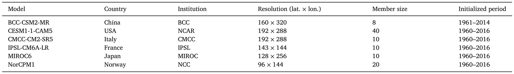
Table 1 CMIP6 DCPP models used in this study.

2.Data and methods

We use the near-surface air temperature of the Component A hindcast experiment of CMIP6 DCPP (dcppA-hindcast) to evaluate the decadal predictive skill for SAT.The models and corresponding information used in this study are listed in Table 1 ( Bethke et al., 2021 ;Boucher et al., 2020 ; Kataoka et al., 2020 ; Nicolì et al., 2023 ; Xin et al.,2019 ; Yeager et al., 2018 ).The surface temperature in the CESM Large Ensemble (CESM-LE; Kay et al., 2015 ) is also used in this study.The monthly mean dataset of the 2-m temperature provided by ERA5( Hersbach et al., 2019 ) is treated as the verification data (OBS).All model datasets are interpolated into a common horizontal resolution of 1°×1°via bilinear interpolation.

Notably, five models initialized every year from 1960 to 2016 predict the following 10 years, except BCC-CSM2-MR, which is initialized from 1961 to 2014 ( Table 1 ) ( Boer et al., 2016 ).The equal weighted ensemble mean of the corresponding initialized members for each model is investigated as signal model results.The multimodel ensemble (MME)is calculated from the unweighted mean of all six models.Since the initialized years end at 2014 in BCC-CSM2-MR, the MME uses a total of 98 ensemble members in the hindcast initialized at the year before 2015 and 90 members after that.The seasonal means are calculated as winter(December–February; DJF), spring (March–May, MAM), summer (June–August, JJA), and autumn (September–November, SON), in which the first year of winter covers January and February.Since there is a significant warming trend in global surface temperature, the 5-year running mean with the linear trend removed is used to extract the decadal signals, where pointXjrepresents the 5-year average from yearj- 2 to yearj+ 2.The lead time represents the time interval between the prediction target and the initial date.The 5-year mean forecasts at lead years 1–5 are investigated in this study.

In this study, the anomaly correlation coefficient (ACC) is used to investigate the skill of the model in capturing the phase of observed variability.The mean-square skill score (MSSS) is also chosen as a deterministic verification metric since it is sensitive to errors in amplitude( Goddard et al., 2012 ).Student’st-test is used to examine the confidence of the ACC with the effective sample size, the formula for which is as follows ( Bretherton et al., 1999 ):

whereNis the number of available time steps, andr1andr2are the autocorrelation coefficients of the two variables lagging by one year.

3.Predictive skill for Eurasian SAT

The “warm Arctic–cold Eurasia ” pattern has attracted considerable attention in the climate research community ( Cohen et al., 2012 ;Mori et al., 2014 ).The spatial pattern of the first leading empirical orthogonal function mode of DJF SAT over the Arctic–northern Eurasia region changed from a uniform warming pattern to a “warm Arctic–cold Eurasia ”pattern around 1998 ( Jin et al., 2020 ).This study investigates the predictive skill for northern Eurasian (40°–70°N, 50°–140°E) SAT since it experienced remarkable decadal variations in recent decades.

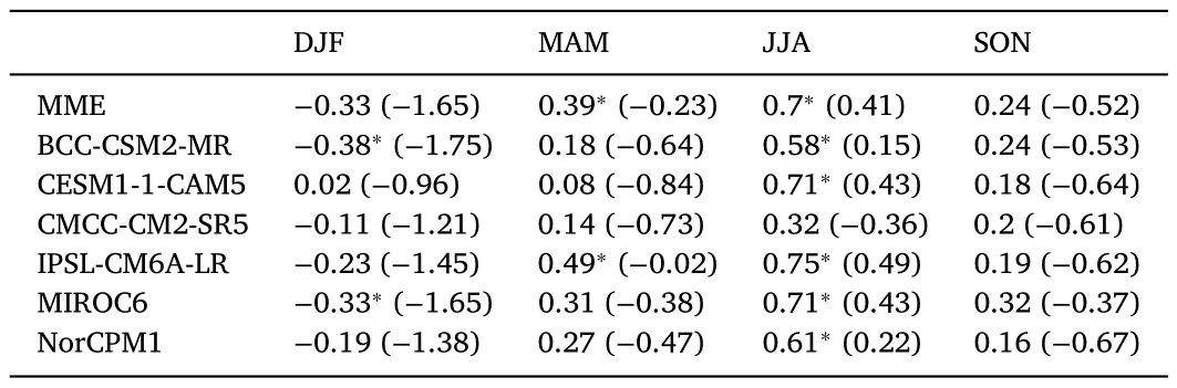
Table 2 The ACC (MSSS) skills for SATI between CMIP6 models and observations in DJF, MAM, JJA, and SON.Values with an asterisk (∗ ) are significant at the greater than 90% confidence level (Student’s t -test).

Fig.1 shows the skills of the models in predicting the seasonal mean Eurasian SAT.Almost no skill can be observed over Eurasia for the winter SAT in the MME and all CMIP6 models.The spring SAT over the Kazakhstan–Mongolia–North China region is well predicted by all six models, in which the MME shows the highest skill.The spring SAT over Russia can barely be predicted by the CMIP6 models, except IPSL-CM6ALR.The six models and MME show significant skill for the summer SAT over the Mongolia–North China region.Except for BCC-CSM2-MR and CESM1-1-CAM5, a certain amount of skill for summer SAT can be observed around Lake Baikal in the remaining models and MME, especially in IPSL-CM6A-LR.The CMIP6 models show limited skill for the autumn SAT over most of Eurasia, apart from in some areas of eastern and northern Russia.

The regionally averaged SAT over Eurasia (40°–70°N, 50°–140°E) is calculated as the SAT index (SATI).The seasonal mean time series of SATI from the model predictions is shown in Fig.2 , and Table 2 displays the skills (in terms of ACCs and MSSSs) for SATI between each model and the observation.

In the observation, there are remarkable decadal variations of winter SATI, such as the positive phase period of 1990–2004 and the negative phase period of 2005–2010.The models generally predict opposite decadal variations of winter SATI than observed, along with a large model spread in the MME.Since all ACCs and MSSSs for winter SATI in the six models are negative, the ACC and MSSS in the MME are - 0.33 and- 1.65, respectively.

The observed spring SATI is generally in a negative phase during 1975–2013 and a positive phase before and after that period, along with remarkable decadal variations.IPSL-CM6A-LR shows a significant ACC of 0.49 compared to the insignificant ACCs in the remaining five models.The MME shows significant ACC skill benefitting from IPSL-CM6ALR.All models have limited skill in predicting the amplitude of decadal spring SATI, all with negative MSSSs.

Except CMCC-CM2-SR5 with its insignificant ACC of 0.32, the other five models show good skill in predicting the decadal variations of summer SATI, with the lowest ACC of 0.58 in BCC-CSM2-MR and highest ACC of 0.75 in IPSL-CM6A-LR.High skill levels in predicting the amplitude of decadal summer SATI are also apparent in IPSL-CM6A-LR,CESM1-1-CAM5, and MIROC6, with MSSSs above 0.42.These skills in BCC-CSM2-MR and CMCC-CM2-SR5 are undesirable, with MSSSs of 0.15 and- 0.36, respectively.The MME also shows reasonable skill for summer SATI, with an ACC of 0.7 and MSSS of 0.41.

Fig.1.ACC skills of between CMIP6 models and observations for Eurasian SAT in (a1–a7) DJF, (b1–b7) MAM, (c1–c7) JJA, and (d1–d7) SON ((a1–d1) MME;(a2–d2) BCC-CSM2-MR; (a3–d3) CESM1-1-CAM5-CMIP5; (a4–d4) CMCC-CM2-SR5; (a5–d5) IPSL-CM6A-LR; (a6–d6) MIROC6; (a7–d7) NorCPM1).Dotted areas are significant at the greater than 90% confidence level (Student’s t -test).

Fig.2.Standardized time series of the MME-predicted (solid blue line) and observed (solid red line) SATI in (a) DJF, (b) MAM, (c) JJA, and (d) SON.The dashed lines denote the SATI predicted by individual models.The skills of the MME in terms of MSSS and ACC are shown in the upper left and right corners, respectively.Values with an asterisk (∗ ) are significant at the 0.1 level (Student’s t -test).The light blue shading shows the model spread in the MME, the interval of which represents the range between the maximum and minimum SATI predicted by all members.

Fig.3.(a–d) ACC skills for Eurasian SAT between CESM-LE and observations.Dotted areas are significant at the greater than 90% confidence level (Student’s t -test).(e–h) ACC skill difference between CESM1–1-CAM5 and CESM-LE.

Table 3 The ACCs of DJF SATI with the MAM/JJA/SON SATI in models and observation.Values with an asterisk (∗ ) are significant at the greater than 90% confidence level (Student’s t -test).

With different atmospheric circulations and external forcings, the autumn SATI shows different decadal variations to the winter SATI( Larkin and Harrison, 2005 ; Abatzoglou and Redmond, 2007 ).The observed autumn SATI also shows significant decadal variations, especially for the period after 1995.All of the ACCs are not significant, and the MSSSs are negative.The models have very limited skills for the autumn SATI, especially for the period after 1985.This is also true in the MME.

Generally, the MME skill for Eurasian SAT is highest in summer, significant in spring, and very limited in winter and autumn.IPSL-CM6ALR has the highest skill in predicting spring and summer SAT.

We further disentangle the impacts of external forcing versus initialization on model skill for Eurasian SAT.The CESM-LE ( Kay et al.,2015 ) has accumulated a 40-member ensemble of historical and projection simulations spanning 1920–2100.CESM1-1-CAM5 was generated using the same code base, component model configurations, and historical and projected radiative forcings as in CESM-LE.The ACC skill difference ( ∆ACC) between CESM1-1-CAM5 and CESM-LE can disentangle the impacts of external forcing versus initialization on hindcast skill ( Yeager et al., 2018 ).Fig.3 shows the ACCs of Eurasian SAT in CESM-LE and the ∆ACC between CESM1-1-CAM5 and CESM-LE.CESMLE shows partial skill for the summer SAT over high latitudes and eastern Kazakhstan where there are negative ∆ACCs, implying that the external forcings account for these skills.However, there are generally positive∆ACCs located over the regions where CESM1-1-CAM5 shows skill for the seasonal Eurasian SAT.This result indicates that the initialization accounts for the current Eurasian SAT skill in CESM1-1-CAM5, which may also be true in other CMIP6 models.

4.Conclusion

The prediction skill for the decadal variability of Eurasian SAT was investigated using large ensemble members from six CMIP6 DCPP models.There are remarkable decadal variations of winter Eurasian SAT.With negative or near-zero ACC skills over most of Eurasia, none of the CIMP6 models has skill for winter Eurasian SAT, for either decadal variations or amplitude.These limited skills also exist for autumn SAT, with insignificant ACCs and negative MSSSs.For spring SAT, the MME has the best skill over the Kazakhstan–Mongolia–North China region, and IPSL-CM6A-LR has the largest significant skill regions over Eurasia.The MME and IPSL-CM6A-LR have skill in predicting the decadal variations of spring SAT, but not for the amplitude given the negative MSSSs.Benefiting from the significant skill over Mongolia and North China, the CMIP6 models show their best skill for the summer Eurasian SAT, excluding CMCC-CM2-SR5 with its large error in amplitude.Compared to external forcings, model initialization accounts more for the Eurasian SAT skill.

Noticeably, the predicted SATIs in the following three seasons seem to show similar decadal variations with that in winter, despite the observed differences being remarkable ( Fig.2 ).We further investigate the predictive skill for the seasonal variations of SATI.Table 3 shows the ACCs between winter SATI and other seasonal SATIs in predictions and the observation.The decadal variability of winter SATI is independent of that in other seasons in the observation.None of the ACCs between the winter SATI and other-season SATIs are significant in the observation.However, the winter situation of a year seems persistent in the following seasons in the CMIP6 models.All ACCs of predicted winter SATI are significantly correlated with the predicted SATIs of other season,excluding CMCC-CM2-SR5 with its remarkable error in JJA SATI.These model system errors should be addressed in future model development.

Funding

This research was funded by the National Natural Science Foundation of China [grant number 41991283 ].