Jia-Hui Song(宋家辉)

College of Science,China Three Gorges University,Yichang 443002,China

Keywords: complex networks,high-order structure,edge importance,connectivity,propagation dynamics

1.Introduction

Some real-world infrastructure systems are subject to targeted attacks and unpredictable failures, which can result in significant financial losses.Understanding the“roles”played by the different components of a system allows us to find the critical components so that we can take advanced measures to protect or increase the resilience of the system.We model realistic complex systems as complex networks whose nodes represent the constituent entities of the system.The edges between them represent the interrelationships between these entities.In this representation, the problem of critical component identification can be easily formulated as quantifying the importance of nodes or edges in the network.There are already many methods to identify important nodes in a network.For example, degree,[1]H-index[2]andk-shell[3]are based on nodes’ neighbors; closeness centrality[4]and betweenness centrality[5]are based on the path; and quasi-Laplacian centrality,[6]the local gravity model[7]and AWLM[8]are based on semi-local structural information.In contrast, the identification and importance ranking of key edges has received less attention.This is because the density of edges in a complex network often determines the complexity of the network, and the sizes of the edges are much larger than those of nodes.Therefore, the contribution of individual edges to the functional properties of the whole network is usually very small,and some subtle changes are difficult to capture.In addition, the contributions from different types of edges to the network are usually interrelated, and this mechanism of “entanglement” in each other makes it difficult to describe their importance individually.These limitations increase the difficulty of critical edge identification to some extent.[9,10]In fact,the identification of critical edges plays an important role in the study of complex networks,as it helps to guide or control the network from a global perspective.First, a network can be made safe from target attacks by protecting critical edges.For example, we can enhance the robustness of a power grid by protecting critical transmission lines.[11]Second, removing critical nodes can be “costly” when we want to suppress the spread of diseases or information.[12]In contrast, strategies that block the path of virus or rumor transmission may be more suitable for certain situations.For example, isolating an airport is an impractical and costly measure,but cutting the route between two locations can be achieved more flexibly and at a lower cost.Current approaches to identifying critical edges focus on the topology of the network.Ballet al.[13]show that the importance of an edge can be measured by the relative amount of change in the average path length of the network after removing that edge.Newmanet al.[14]used edge medial centrality (EB) to quantify the importance of edges.Yuet al.[15]proposed a method named BCCMODwhich calculates the number of clusters on an edge considering that the greater the number of clusters an edge belongs to, the less important it is.However, it is not applicable to large-scale networks because it is time-consuming.Subsequently, many researchers started to use local information to describe the importance of edges in order to reduce the time complexity.For example, Kanwaret al.[16]proposed a metric namedECDCNusing the betweenness of edges,the degree of nodes at both ends of the edge and the number of common neighbors.Simulation results show that the method has a low time complexity to quickly identify the key edges in large networks.However, the accuracy of this metric is low because it only considers the situation within the first-order neighborhood.Holmeet al.[17]assumed that edges between important nodes in the network are more important than other edges and proposed the degree product (DP) index to evaluate the importance of edges.Onnelaet al.[18]proposed the topological overlap (TO) to quantify the effect of common neighbors of nodes on the importance of edges.Chenget al.[19]found that the nodes at both ends of an edge in a small cluster that are also in a large cluster are important for the connectivity of the network and proposed the bridge degree(BN)index.Liuet al.[20]proposed diffusion intensity (DI) to identify critical edges from the perspective of diffusion dynamics.Matamalaset al.[21]considered the characteristics or parameters of the epidemic transmission process and proposed a set of discretetime control equations(ELE)that can be closed and analyzed to evaluate the contribution of links to the propagation process in complex networks.This also provides a new way of thinking to analyze dynamic diffusion models at the link rather than node level.Xiaet al.[22]proposed an importance metric that can be used to quantify a single edge or a set of edges based on the connectivity of nearest neighbors of nodes.Renet al.[23]proposed an edge ranking algorithm that considers both local and global information by combining the node influence distribution law and the irreplaceability of edges.Chenet al.[24]proposed a novel and effective sub-graph overlap(SO)metric based on the degree of overlap of communities within an edge neighborhood.This method can identify the key edges that maintain the“communication”between different communities(tightly connected sub-networks) in the network.However,this metric is more suitable for networks with a high degree of modularity and is less accurate in the face of homogeneous networks with a high link density of edges.Zhaoet al.[25]considered the second-order neighborhoods of the nodes at both ends of an edge and proposed a second-order neighborhood(SN)index to quantify the role played by an edge in maintaining network connectivity.TheSNfaces a similar problem to theSOin not being able to identify the important edges of a high-density homogeneous network.It can be seen that the current edge importance metrics focus on identifying“bridge edges”between communities in heterogeneous networks with high modularity,but not for homogeneous networks with high link density.In this paper, we summarize the shortcomings of the above studies and propose an edge importance metric based on the number of higher-order structures within the first and second-order neighborhoods of an edge to identify the important edges in a homogeneous network.In addition to the triangles in the first-order neighborhood of the edge,the fully connected quadrilateral and diagonal quadrilateral in the firstorder neighborhood of the edge and the empty quadrilateral and diagonal quadrilateral in the second-order neighborhood are also taken into account,so that the higher-order structures considered are more diverse and richer in variety.The importance of edges in the global position of the network is also considered.The main idea of this metric is that the removal of edges from the network causes a decrease in the connectivity and propagation capacity of the network structure,and has an impact on the integrity of the network structure.We use this metric as a measure to compare with the current representative measures of edge importanceECDCN,SOandSNmetrics.The effectiveness of the metric is verified in six networks by five aspects: the SI model, robustness metricR, number of connected branchesθ,Kendall’s tau correlation coefficientτ, and monotonicityM(R).The numerical simulation results show that the proposed edge importance metric can identify the edges that have the greatest influence on the network structure and function more quickly and accurately.

The paper is structured as follows.In the first part, a brief introduction is given to the basic concepts of complex networks and the three edge importance measures that are currently most popular for comparison, along with new definitions of higher-order structures on edges, first and secondorder neighborhoods of edges, and the concepts of inner and outer edges.In the second part, the new measures for evaluating edge importance are introduced.In the third section,the data set used is described and simulations are performed in six networks to derive the superiority of the proposed metric.Finally, we conclude with a summary of the work done and some prospects for future research.

2.Centrality measure

Before we start,we introduce the basic concepts of complex networks.The complex network can be represented byG=(V,E), whereGis an undirected connected graph, withnnodes,medges,Vrepresents the set of nodes,Erepresents the set of edges, the adjacency matrix ofGofQ=[aij] hasnrows andncolumns, and the elements inQare defined byaijas follows: (i)aij=1,theith node is connected to thejth node;(ii)aij=0,theith node is infinitely connected to thejth node.

2.1. ECDCN

In a complex network, the following information is required in order to identify a critical edge and properly quantify its diffusion capacity.

1○The global position of the edge in the network.

2○Local topological features in the network that promote diffusion through that edge.

3○Local topological features that suppress diffusion through this edge in the network.

Based on this,Kanwaret al.proposed a hybrid edge centrality metric that combines edge betweenness,the product of node degrees at both ends of the edge and the number of common neighbors.It is defined as

whereuandvrepresent the two end nodes on the edge, and this edge is denoted bye=(u,v).It locates an edge through a global perspective using the edge betweennessBC(u,v).The local topological features that facilitate diffusion through edgeeare represented by the degree productDP(u,v) of nodesuandv.To quantify the local topological features that impede the diffusion of edgee, we use the common neighbor countsCN(u,v)of nodesuandv.The time complexity of this metric isO(|V||E|).[16]

2.2. SO

The literature[25,26]states that a common edge between two different communities in a network is often more important than an edge within a community in facilitating communication between communities in the network.Based on this,Chenet al.describe the importance of edges based on the degree of overlap of communities within an edge neighborhood.For a given static networkGand an edgeei j, there is a subgraph ofGthat contains nodesi,jand nodes whose distance fromiorjis not greater than 2.TheSOmetric is defined as

2.3. SN

If nodeiand nodejhave few second-order common neighbors,edgeeijis more likely to be a potential“bridge”between two different communities,which is essential to facilitate communication between them.[25,26]Therefore,the smaller theSNindex,the more important the role played by edges.The computational complexity ofSNisO(M〈k〉),whereMis the number of edges and〈k〉is the average degree.[23]

2.4.Higher-order structures on the edge

Networks are inherently limited to describing pairwise interactions, whereas real-world systems are usually characterized by higher-order interactions involving three or more units.Therefore,higher-order structures,such as hypergraphs and simple complex shapes, are better tools for depicting the real structure of many social, biological, and man-made systems.[27]A triangle is the smallest higher-order structure,which is a third-order (node number 3) connected subgraph formed by three edges interconnected at the beginning and end.It serves as the basic component unit of the association and the basic topology of the network.The size of the higherorder structure is between a single node and a large dense association.It is a fully or partially connected subgraph consisting of a few nodes connected in a guaranteed closed loop, and it appears more frequently in real networks than in their corresponding random networks,and increases with the size of the network and the density of connections between nodes.There are five main cases of third and fourth-order structures of an edgeein its first and second-order neighborhoods (with the number of nodes 3 and 4).Here the first-order neighborhood of an edgeeis the set of nodes whose maximum distance from the two end nodes ofeis 1, and the second-order neighborhood ofeis the set of nodes whose maximum distance from the two end nodes ofeis 2(for simplicity,we assume that the distance between two directly connected nodes is 1).If the maximum distance of all nodes except nodei,jfromi,jon the higher-order structure witheijas one side is 1, then the higher-order structure is said to be in the first-order neighborhood ofeij.If the maximum distance of all the nodes except nodei,jfromi,jon the higher-order structure witheijas one side is 2, then the higher-order structure is said to be located in the second-order neighborhood ofei j.As shown in Fig.1, 1○–5○are the third-order and fourth-order structures within the first-order and second-order neighborhoods of edgeeij, respectively.From Fig.1, we can see that in 1○, 2○, 4○and 5○,the break of edgeei jcauses the higher-order structure to change from a closed state to an open state.In 3○, however, the disconnection ofei jdoes not cause the higher-order structure to change from closed to open.In fact,in the neural network of the brain,even ifei jis disconnected in 3○,a basic functional module can still be maintained; for example,basic information transformation and storage can still be completed.However, the disconnection of edgeei jin 1○, 2○, 4○and 5○results in the loss of this specific function.[28–30]However,we can be sure that in 1○–5○, the disconnection ofei jmakes the shortest path length fromi →jlarger in all cases.This predicts a decrease in communication or transmission efficiency in communication networks and grids.[31–34]We refer toeijin the first case as the outer edge andei jin the second case as the inner edge.The inner and outer edges play different“roles”in different complex environments.Furthermore,these five specific higher-order structures within the first-and second-order neighborhoods of the edges considered in this paper have different roles in different real-world complex systems.Some can reflect the resilience level of the system and serve as an early warning of system failure or risk, while others play an irreplaceable role in the functionality of the system.For example,in financial networks the decrease in the number of 1○, 4○(fully connected)types predicts possible financial risks and in infrastructure networks the number of 1○, 4○types can reflect the vulnerability of the network at a certain level,[35,36]while in biological networks the sudden change in the number of 2○, 3○(partially connected)types is considered as a precursor of cellular carcinogenesis[37,38]and the structure of 5○(loop)types in neural networks of the brain assume important functions such as storage and transformation of information.[39,40]Therefore,we consider them together in combination.

Fig.1.1○–5○denote the higher-order structures in the first-order and second-order neighborhoods of edge eij, where 1○denotes a triangle in the eij first-order neighborhood, 2○denotes a diagonal quadrilateral in the eij second-order neighborhood, 3○, 4○denotes a diagonal quadrilateral and a fully connected quadrilateral in the eij first-order neighborhood, and 5○denotes an empty quadrilateral in the ei j secondorder neighborhood.

3.Proposed method

This paper proposes an edge importance measure, i.e.,edge clustering coefficients, and extends it to the secondorder neighborhood.The scope is extended from the firstorder neighborhood of edges to the second-order neighborhood, and the types of higher-order structures are extended from a single triangle to a diagonal quadrilateral, fully connected quadrilateral, and empty quadrilateral.The effects of triangles, diagonal quadrilaterals, fully connected quadrilaterals and empty quadrilaterals on the network topology and propagation dynamics are considered comprehensively.The effect of edges on the global characteristics of the network(average path length)is also considered.The equation for this metric is expressed as follows:

whereki,kjare the degrees of nodesi,j, respectively.NΔ=(ki+kj-2) denotes the maximum possible number of triangles in a first-order neighborhood witheijas the outer edge.Nα=(ki-1)(kj-1) denotes the maximum possible number of empty quadrilaterals in a second-order neighborhood thought to be the outer edge ofeij.Nβ=(NΔ/2) denotes the maximum possible number of diagonal quadrilaterals in the first-order neighborhood witheijas the inner edge.Nη=(ki+kj-2)(ki+kj-3)denotes the maximum possible number of diagonal quadrilaterals in the second-order neighborhood witheijas the outer edge.N■=(NΔ/2)denotes the maximum possible number of fully connected quadrilaterals in the first-order neighborhood witheijas the outer edge.In summary, the denominator represents the sum of the maximum number of triangles, diagonal quadrilaterals, fully connected quadrilaterals and empty quadrilaterals in the first and secondorder neighborhoods witheijas the inner and outer edges in the ideal case.LetΓi∖jbe the set of nodes in the first-order

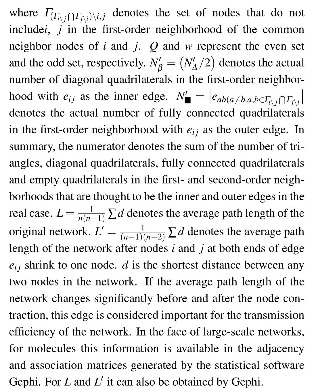
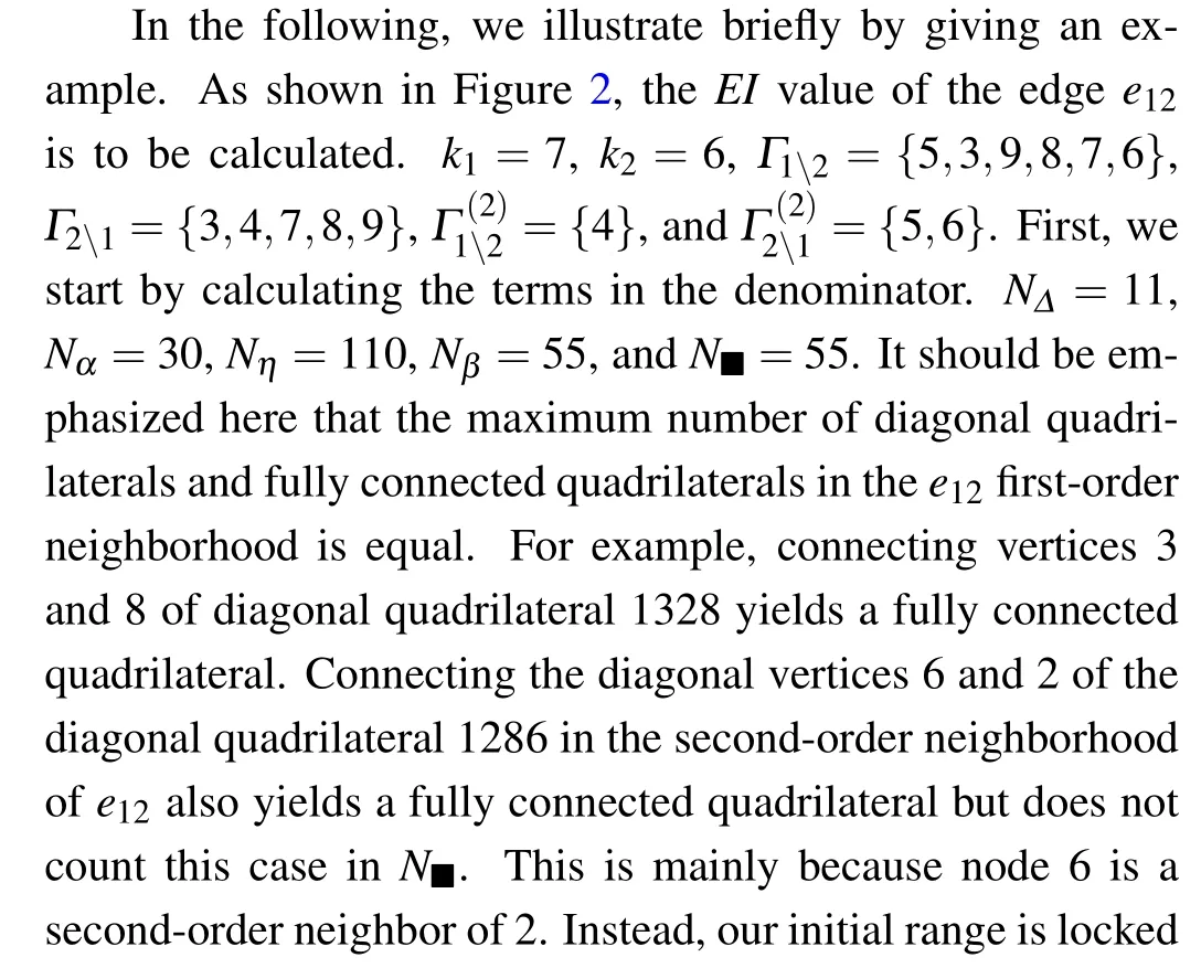
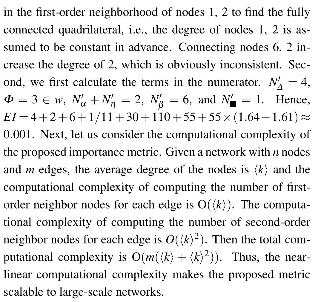
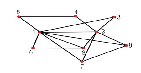
Fig.2.Toy network.

4.Experimental setup

4.1.Data sets

In order to test the effectiveness of the proposed method,we apply it to real-world networks and artificial networks.Real-world networks include (i) electricity: the network of power grids;(ii)network science:the coauthor network in network science consists of 1589 nodes and we choose the largest dense community of 400 nodes in this network;(iii)email:the email network of the University Rovirai Virgili;and(iv)yeast:the protein–protein interaction network.These data sets are available from: http://vlado.fmf.uni-lj.si/pub/networks/data/.Table 1 shows the statistical characteristics of four networks of different sizes.The two artificial networks are WS small world network and BA scale-free network.First,a small world network is constructed,in which nodesn=1000,linksm=1475,and nodes are connected with a probability ofp=0.01.The average degree of the network is〈k〉≈3.The scale-free network takesN=1000,m0=5,m=4(for the initial network withm0nodes,each time a new node is introduced to connect withmexisting nodes,m ≤m0), and generates a scale-free network withN=1000 nodes andmt=3980 edges (tsteps are required to generate the required scale-free network).In this paper,all these real-world networks and analog networks are regarded as undirected and unweighted.

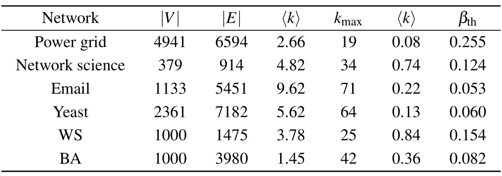
Table 1.Some statistical properties of four networks.Topological features include: number of nodes (|V|), number of edges (|E|), average degree (〈k〉), maximum degree (kmax), average clustering coefficient(〈k〉),and propagation threshold(βth=〈k〉/〈k〉).

4.2.Evaluation methodology

4.2.1.SI model

To compare the accuracy of the proposed metric in identifying the propagation ability of edges,the SI model is used to simulate the propagation and evolution in real networks.The SI model contains only two types of nodes,susceptible nodes(S)and infected nodes(I).Once a node is infected,it is never able to recover.As the time increases,the number of infected nodes in the network increases until all nodes are infected and the process stops.In our experiments,we keep the propagation rate exactly above the propagation threshold of the epidemic in the networkβth.The experiment starts with any one node in the network as an infected node and the number of infected nodes in the network after 100 time steps isF(t1),which can be used to reflect the propagation ability of the nodes in the network.The formula is as follows:

whereM=200 is the total number of experimental repetitions.f(m)=n/Nis the proportion of infected nodes in the network after 100 time steps for each experiment,nis the number of infected nodes in the network after 100 time steps for each experiment, andNis the total number of nodes in the network.We rank the edges in the network from largest to smallest according to the four edge importance measures,EI,ECDCN,SO,andSN, and select the top 20 percent of edges for each.The edges are removed from the network sequentially starting from 100 time steps,and 2 percent of the top 20 percent of the edges are removed at each time step.After 50 time steps(when the top 20 percent of edges are removed),let the proportion of infected nodes in the network beF′(t2).The same experiment is conducted 200 times to take the average value.We then defineρas

where 0≤ρ ≤1.From the perspective of propagation dynamics,the greater the influence of an edge,the greater the ability of that edge to be removed from the network to inhibit proliferation,and the fewer the number of nodes in the network that end up in the infected state,i.e.,the smallerρ.

4.2.2.RobustnessR

The performance of EI is evaluated by an edge percolation process.[30,31]Edges are sequentially removed from the network according to the ranking results of the four edge importance metricsEI,ECDCN,SO, andSNand the greater the change in the topology of the network after removing the same proportion of edges, the more important the removed edges are.In this paper, the impact on network connectivity after edge removal is evaluated by the robustness metricR.[32]The formula is defined as

wheremrdenotes the number of edges removed andmdenotes the total number of edges in the network.δ(mr/m)denotes the proportion of nodes in the largest connected branch in the network after removingmr/mproportion of edges.Obviously,a smallerRindicates that the metric can better destroy the connectivity of the network, which means it can better rank the importance of edges.

4.2.3.Number of connected componentsθ

The number of connected components is an indicator of the degree of “fragmentation” of the network, i.e., the extent to which the network structure is disrupted.The original network has a relatively complete structure where most nodes are located on a giant connected branch, and the number of connected branches in the network is small.As we perform edge removal,the number of connected branches in the network increases gradually as the giant connected branches are cut off and broken into many smaller connected branches.We also rank the edges in the network from largest to smallest according to the four edge importance measuresEI,ECDCN,SO,andSNand each select the top 50(p=50%)percent of edges for removal.We observe the number of connected branches in the final network.

4.2.4.Kendall’s tau correlation coefficientτ

Kendall’s tau correlation coefficient is selected to determine the consistency between the ranking list obtained by the specific measurement method and theF(tc) ranking list obtained by the SI model.Given two ranking listsXandY,(xi,yi) and (xj,yj) are the two edge pairs in these lists.The Kendall tau correlation coefficient is defined as

In this paper,Xrepresents the ranking result of edges obtained from a centrality measure,andYrepresents the ranking result of the number of infected nodes obtained from the SI model.Ifxi ＞xj,yi ＞yjorxi ＜xj,yi ＜yj,we say that the ordering ofxiinXand the ordering ofyiinYare the same.Otherwise,it is called inconsistent.n1andn2represent the number of consistent and inconsistent pairs,respectively,andNis the length of the sorting listX.Obviously,τis between-1 and 1.Here,τ=-1 means that the order of these two lists is completely opposite.At that time,τ=1, the order of the two lists is the same.

4.2.5.MonotonicityM(R)

In order to distinguish the propagation ability of all edges,each edge should be assigned a unique indicator through centrality measurement.The proportion of repeating elements in a sequence is called the monotonicity of the sequence.In order to quantify the monotonicity of different sorting methods,we useM(R)[8]and define it as

whereNis the length of the ranking listR,Nrindicating the number of edges with the same sorting valueR.The range ofMvalues is 0 to 1.The best value ofMis 1,which means that each edge in the network has a unique and identifiable sorting value.In contrast,the worst value ofMis 0,which means that all edges in the network have the same ranking.

4.3.Experimental results and analysis

In the experiments,the proposed edge importance metric is compared with three other metrics, includingECDCN,SO,andSN.We use different methods to analyze the performance of the proposed centrality metric in terms of propagation ability,robustness,etc.

4.3.1.Spread capacity analysis

The simulation results of the four metrics on six networks are shown in Fig.3.It can be seen that in(a)–(e),theEImetric always makespthe smallest, i.e., the smallest number of nodes eventually infected.In (f),ECDCNoutperformsEIby about 110 time steps; this is because nodes with larger betweenness or degree in BA networks are generally the“hubs”in the network, andECDCNhas the advantage of identifying the edges connecting nodes with large degree or larger betweenness nodes in the network.For BA networks, once the“hub”node is infected,the spread of the disease is accelerated.The ability ofECDCNto identify the links connected to the“hub”nodes and block them in time slows down the spread of the disease to some extent.However,as time increases,it can be seen thatEIoutperformsECDCNand gradually closes the gap.This is because as the degree of the“hub”node decreases the network becomes more homogeneous,and the effect ofEIgradually emerges.At the same time,it can be seen thatEIis more effective in the face of high-density homogeneous networks.In addition,we can also see that the suppression effect ofSOandSNon propagation is approximately equal.This is because both are metrics used to identify links between different communities in the network.From (b) and (e), it can be seen that the suppression effect ofSOandSNis second only toEI.This is because the modularity of network science and WS networks is higher as there are more communities in the network;SOandSNcan identify the links between communities and cutting these links will make the virus only spread within the community.In Fig.4, the same result can be seen after 150 time steps(d)i.e.theEImetric makes the network infected with the least number of nodes.In summary,we can conclude that theEImetric can be effective in identifying important edges in the propagation process.

Fig.3.The ρ as a function of t.The changes in infected nodes in the six networks with the continuous removal of edges are obtained by averaging the results over 200 independent simulations of the SI model for each network,with β slightly larger than βth.

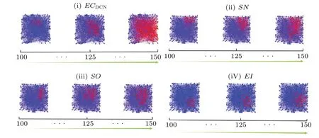
Fig.4.The visualization result of SI model on network science.The blue nodes are susceptible states and the red nodes are infected states.Each of them corresponds to an edge importance metric.

4.3.2.Robustness

The simulation results of the four metrics on the six networks are shown in Fig.5.It can be seen that in (a)–(f)EIis always the fastest decreasing as the proportion of edge removal increases.In (b),SOoutperformsEIuntilδdrops to 0.55, andSNoutperformsEIuntilδdrops to 0.64.This is because network science contains more communities, soSOandSNcan identify the links connecting different communities and disconnect them in the early stage, which can cause great damage to the connectivity of the network.However,withδat[0,0.55]and[0,0.64],it can be seen thatEIis always better thanSOandSN.SOandSNcannot accurately identify edges in these sub-networks,so the damage to the connectivity of the network is gradually diminished.Similarly, we can see the same phenomenon in (e).Forδin [0, 0.62] and [0,0.67],SNandSOoutperformEI,but in[0.62,1.0]and[0.67,1.0]EIis always better thanSOandSN.In (f),ECDCNoutperformsEIat[0, 0.7]becauseECDCNis able to identify the links attached to the“hub”nodes and remove them in time.As the number of links connected to the “hub” nodes decreases,the network is gradually “fragmented” into many small clusters,which can cause some damage to the connectivity of the network in a short period of time.Since the degree of heterogeneity of nodes in these small clusters is low and there are no nodes with large degrees or meshes,ECDCNcannot accurately identify the edges connected to nodes with large degrees or betweenness.Thus we see thatEIis always better thanECDCNwhenδis between[0.7,1.0].To more accurately illustrate the computational merits of the proposed metric, we remove the top ten percent of edges from the network at each time step Δtaccording to the ranking results of the four edge importance metrics and observe the time taken to finally minimize the maximum connected branches of the network.

Fig.5.Ratio of nodes on the largest connected branch as δ function of the ratio of edges removed p.Ratio of nodes of the largest connected component after removing p ratio of edges in six networks.Results obtained by averaging 200 independent simulations for each network.

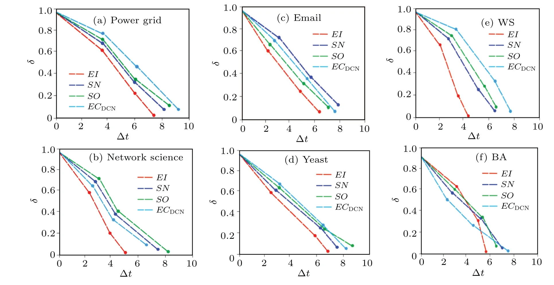
Fig.6.Ratio of nodes on the maximum connected branch δ as a function of time step Δt on six networks.Each network is the result obtained by averaging 100 independent simulations on MATLAB.

As can be seen in Fig.6,the edge metricEIalways takes the least time to maximize the decomposition of the connected branches in these six networks, with the best performance ofEIin network science and WS taking the least time.This is mainly due to the larger link density and average clustering coefficient of the two networks,which also confirms our previous statement thatEIperforms better in the face of high-density homogeneous networks.In addition, the computational efficiency ofSO,SN,andECDCNis different in each network and the computational superiority in each network is also different,which is mainly due to the different topological characteristics of different networks, so we do not elaborate too much here.All the results show that decomposing the network according to the ranking results of the edge importance measureEIcan destroy the robustness of the network the fastest.

4.3.3.Number of connected branches

The simulation results of the four metrics on the six networks are shown in Fig.7.It can be seen in (a), (c), (d) that as the proportion of edge removal keeps increasing,EIalways makes the number of connected branches in the network increase fastest and eventually the most.In(b),SNandSOare superior toEIforθat [0, 0.07], [0, 0.13].This is because network science contains more associations, andSNandSOpreferentially identify links connecting different communities to each other.The removal of these links leads to a rapid increase in the number of connected branches (small associations)in the network in a short period of time.Afterp=0.07,0.13 the removal of edges is concentrated in each community and the disruptive effect ofSNandSOon network connectivity is reduced,soEIis always superior toSNandSO.Similarly,in(f),ECDCNoutperformsEIwhenpis within[0,0.15],thanks to its ability to identify links connected to“hub”nodes and remove them in a timely manner.The gradual“fragmentation”of the network into smaller clusters leads to an increase in the number of connected branches.Afterp=0.15,the removal of edges is concentrated in each small dense homogeneous cluster, and it can be seen thatEIgradually outperformsECDCN.The computational efficiency of the proposed metric in terms of decomposing the network is similarly observed by removing the top ten percent of the ranked edges sequentially from the network at each time step Δtaccording to the ranking results of the four edge importance metrics, and separately observing the time used to reach a certain number(in the vicinity of this number)of connected branches in each network.Here we set the fixed number of connected branches to be reached in each network as 2000, 200, 500, 1000, 600 and 600, respectively.The results are shown in Fig.8,which shows that the use of the metricEIto remove edges results in the shortest time to reach a fixed value for the number of connected branches in the six networks,with the best performance in network science and WS.This confirms the conclusion of Subsection 4.3.2 and reflects that the proposed metricEIcan quickly and accurately identify the important edges in the “skeleton”of the network,which are the basis for the derivation and development of the network.In addition, the three metricsSO,SNandECDCNhave their own advantages and disadvantages in each network.In the BA network, it can be seen that the decomposition efficiency ofECDCNbefore Δt=4 is still very high, which is mainly due to the special topological characteristics of the BA network as mentioned before.In summary,the edge importance metricEIcan effectively and efficiently disrupt the structure of the network.

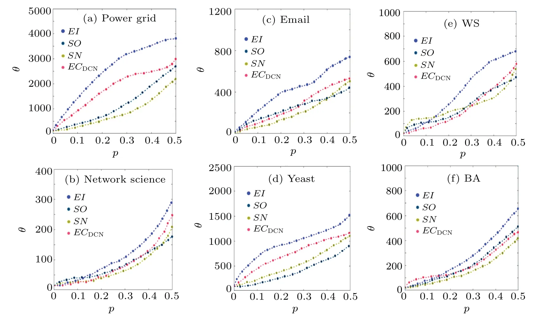
Fig.7.Number of connected branches θ as a function of the edge removal ratio p.Each network is the result of averaging 200 independent simulations.

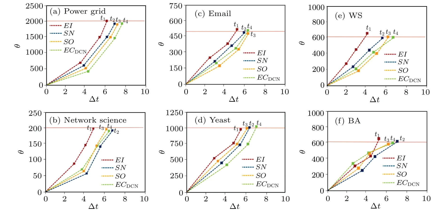
Fig.8.Number of connected branches θ as a function of time step Δt on six networks.Each network is the result obtained by averaging 100 independent simulations on MATLAB.

4.3.4.Analysis of BA scale-free networks

The simulation results in Subsections 4.3.1, 4.3.2 and 4.3.3 show that the performance of the proposed metricEIfor BA networks is less satisfactory in the early stage, while the performance ofECDCNin the early stage is superior compared to the other three metrics.We have emphasized earlier that this is due to the special topological properties of BA networks, and here we analyze these two points in more detail.A random scale-free network with 600 nodes and 2760 edges is constructed using the Python networkx package as an example,where the network has three communities and two hub nodes.As shown in Fig.9,Arepresents the largest community andCrepresents the smallest community.In the propagation experiment in Subsection 4.3.1,at the initial moment we randomly select a node from the network as the source of infection and start the edge removal operation after 100 time steps.In BA networks, nodes with a large betweenness or degree are generally hubs in the network, through which the virus can propagate to various communities and eventually cause widespread infection, whileECDCNhas the advantage of being able to identify the edges connecting nodes with a large degree or large betweenness in the network.As these edges are removed so that the virus cannot spread to other communities in the network but is restricted to the local area(in its own community), we can see that the inhibitory effect on propagation in the early stage is better thanEI.With the removal of edges, the link between the hub node and each community gradually decreases and the network is broken down into several high-density homogeneous small communities;at this time the superiority ofEIbecomes apparent,so the inhibitory effect on propagation is better thanECDCNin the later stage.Also in Subsections 4.3.2 and 4.3.3, the initial network as a whole has only one maximum connected branch, and as we gradually remove the edges identified byECDCNthis causes a sharp decrease in the number of nodes on the maximum connected branch and a rapid increase in the number of connected branches in a relatively short period of time,as the network is disintegrated into many smaller communities and a number of isolated nodes.However,the metricEIcomes into play as the focus of work gradually shifts to each community.Although the proposed metricEIworks better in the face of homogeneous networks, we can also adapt it to heterogeneous networks better by making appropriate modifications to the formula.The modified formula is defined as

wheremstis the total number of shortest paths between nodessandt, andmst(ei j) represents the number of these paths through edgeeij.That is, ∑s/=t mst(ei j)/mstrepresents the global betweenness of edgeei j.BiandBjdenote the betweenness of the nodes at each end of edgeei j, respectively.In this formulation we consider some special properties of importance edges in the face of heterogeneous networks.First,when the betweenness of edgeei jis larger it indicates that it may be a bridge edge connecting communities to each other.Secondly, when the absolute value of the betweenness of the nodes at both ends of edgeeijis larger it indicates that one of the nodes may be a bridge node between communities.In fact,the introduction of these two points does not increase the complexity of the original computation because the edge and node betweenness can be obtained from the network statistics software Gephi.In the following, we compare the modified metric EII withEIandECDCNin three aspects (propagation capability,robustness,and number of connected branches)on the BA network of Table 1.The results are shown in Fig.10,which shows that EII always outperformsECDCNin (a)–(c)and performs more consistently thanEIthroughout.Therefore, in practical applications, the appropriate metric should be selected according to the topological characteristics of the network under testing.

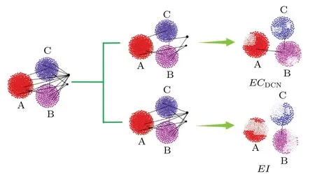
Fig.9.The EI,ECDCN visualization of the evolutionary process of two metrics applied on a random scale-free network,where three moment images in the time configuration window are intercepted.The size of the white area represents how the community has been broken down internally.

Fig.10.Comparison of the three metrics EII,EI and ECDCN,where each BA network is the result of averaging 200 independent simulations.

4.3.5.Kendall’s tau correlation coefficient

In order to test the accuracy of the proposed centrality measure, it is compared with three different centrality measures on six networks under the SI model.Theoretically, the closer the value ofτis to 1,the better the performance of the sorting method.The selection valueβthchanges near the epidemic threshold.The valueβthis related to the topological characteristics of a given network, so the abscissa of different networks in Fig.11 is different.Figure 11 describes the Kendall’s tau correlation coefficient of four central indicators varying with the probability of infection.As shown in(a)–(f),the value ofτforEIis always the largest.In(b)and(e),SOandSNhave the second highestτ-value afterEI.this is because there are more associations in network science and WS networks,andSOandSNcan identify the links between communities.However, after the links between communities are identified,SOandSNthen start to identify the links in each association leading to a decrease in accuracy.Thus, it can be seen that the consistency between the ranked lists of both metrics is from strong to weak.In (f), theτ-value ofECDCNis second only toEIand at [0.11, 0.16] they are approximately equal.This is becauseECDCNis able to identify edges in BA networks connecting nodes of large degree or larger betweenness.However,after the links with large degree are identified,the accuracy of identification decreases because the degrees of all nodes in the BA network except the“hub”node are not very different,so we can see that the consistency is gradually weakening.

Fig.11.Kendall’s tau correlation coefficient(τ)between the ranking results obtained from the four different metrics and the F(t)ranking list obtained from the SI model with different infection probabilities β. β changes near the neighborhood of βth.Results obtained by averaging 100 independent simulations of the SI model.

4.3.6.Analysis of monotonicity

A good centrality measure should be able to distinguish between edges with different propagation capabilities.Table 2 shows the monotonicity of the four centrality measures in six different networks.The closerMis to 1,the better the performance of the centrality measure is.It can be seen that among the four centrality measures, the monotonicity value ofEIis always close to 1 in all networks.In summary,EIcan better distinguish edges with different propagation capabilities.

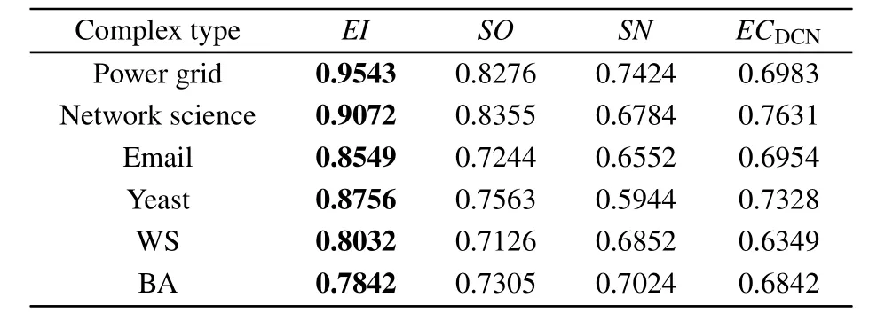
Table 2.Monotonicity of four centrality measures in six networks.

5.Conclusion

This paper proposes a new edge importance metric for identifying the most influential edges in a network.The metric innovatively considers loops and diagonal quadrilaterals in the second-order neighborhood of edges as well as fully connected quadrilaterals and diagonal quadrilaterals in the firstorder neighborhood.Moreover,the higher-order clustering coefficients of edges are defined.We consider that the removal of edges affects the connectivity and completeness of the local structure of the network.The superiority of the proposed metric is obtained by simulating the actual network.This paper innovatively introduces the idea of probability for the first time to identify higher-order structures within edge neighborhoods,which provides a powerful analytical tool for future developments in the field of network science and hopefully will see more integration between the two fields.Furthermore, only higher-order forms within the first and second-order neighborhoods of edges are considered in this paper.In fact, as the scope of the analysis (the neighborhood of the edge) is extended outward,we see that the variety of higher-order structures grows exponentially in richness far beyond our imagination.How will the new structures that emerge in this section affect the structure and function of the network? This work will be explored in the next step.In the meantime, we will also propose some targeted protection strategies for the higherorder organization of the network.