Dayong WEN and Jie CAO

Yunnan Key Laboratory of Meteorological Disasters and Climate Resources in the Greater Mekong Subregion,Yunnan University, Kunming 650091, China

ABSTRACT Based on the fifth-generation reanalysis dataset from the European Centre for Medium-Range Weather Forecasts for 1979—2019, we investigated the effects of the circumglobal teleconnection (CGT) on the interdecadal variation of the March atmospheric heat source (AHS) over the Southeast Asian low-latitude highlands (SEALLH).The dominant mode of the March AHS over the SEALLH features a monopole structure with an 8—11-year period.Decadal variations in the AHS make an important contribution to the 11-year low-pass filtered component of the AHS index, whichexplains 54.3% of the total variance.The CGT shows a clear interdecadal variation, which explains 59.3% of the total variance.The March AHS over the SEALLH is significantly related to the CGT on interdecadal timescales.When the CGT is optimally excited by a significant cyclonic vorticity source near northern Africa (i.e., in its positive phase), the SEALLH is dominated by anomalous southerly winds and ascending motions on the east of the anomalous cyclone.The enhanced advection and upward transfer result in a high-enthalpy air mass that converges into and condenses over the SEALLH, leading to a largerthan-average March AHS over this region.The key physical processes revealed by this diagnostic analysis are supported by numerical experiments.

Key words: interdecadal variation, atmospheric heat source, circumglobal teleconnection, low-latitude highlands, Rossby wave source

1.Introduction

Low-latitude highlands are located between 30°S and 30°N and have an average elevation of at least 1000 m.Ten low-latitude highlands, including the Southeast Asian low-latitude highlands (SEALLH; 18°—30°N, 96°—108°E), meet these criteria worldwide (Qin and Ju, 1997; Xie and Liu,1998).The SEALLH mainly includes the Yun—Gui Plateau and its southern extension in northeastern Myanmar, northern Laos, and northern Vietnam (Fig.1).The SEALLH has its highest and lowest elevations in its northwestern and southeastern parts, respectively.The SEALLH and its meridional mountains and rivers cover an area of approximately 9 ×105km2, about one-third of the size of the Tibetan Plateau(TP).Its complex landforms and distinctive geographical position result in water vapor from the tropical Indian Ocean and tropical western Pacific mixing over the SEALLH and entering the East Asian monsoon region (Holmes et al.,2009; Cao et al., 2012, 2016; Tao et al., 2016).In this way,at least to some extent, the SEALLH modulates the weather and climate over East Asia (Chang et al., 2005; Xie et al.,2006; Meng et al., 2014).

In comparison with the numerous studies of the atmospheric heat source (AHS) over the TP and its effects (Son et al., 2019, 2020), since the pioneering studies of Yeh et al.(1957) and Flohn (1957), there have been relatively few studies of the AHS over the SEALLH adjacent to the TP.The SEALLH and southern margin of the TP are characterized by a large average annual heat flux of >200 W m—2, equivalent to that of tropical convection (Fig.2a).The AHS in the SEALLH exhibits a clear annual cycle, with larger variability from November to April.Given that the SEALLH generally transitions from a heat sink to a heat source in March, one month earlier than that of the TP, it is one of the earliest AHS to develop in the East Asian summer monsoon region(Fig.2b).Previous studies show that the land—sea thermal contrast between the region south of the SEALLH and its surrounding oceans in spring can be a precursory signal of the South China Sea summer monsoon onset (Xu et al., 2002;Chow et al., 2006; Li et al., 2020; Zhuang et al., 2022).The earlier the atmospheric heat source over the region south of the SEALLH becomes persistently greater than that compared to the South China Sea, the earlier the summer monsoon establishes itself over the South China Sea (Liu et al., 2010; Zhu and Li, 2017).The AHS variability of the SEALLH in its transition month may provide possible theoretical guidance for understanding the establishment of the summer monsoon.However, the variability of the March AHS over the SEALLH and what causes these variations remain unclear.

The circumglobal teleconnection (CGT) with a wavenumber five structure in the upper-tropospheric meridional wind and streamfunction fields is a hemispheric-scale, low-frequency pattern that propagates along with the waveguide for Rossby waves in the boreal winter (Hsu and Lin, 1992;Hoskins and Ambrizzi, 1993; Branstator, 2002).The CGT is an important factor that affects the temperature, precipitation, and extreme weather in East Asia (Huang et al., 2011;Yuan et al., 2015; Wu et al., 2016b).Recently, some studies have suggested that the CGT undergoes significant interdecadal variations (Wang et al., 2012; Wu et al., 2016a, b,2019).Therefore, an important unresolved issue is whether the CGT modulates the March AHS over the SEALLH,along with what key physical processes link the CGT and March AHS.This study was undertaken to address these two issues.

2.Data and Methods

2.1.Data

The datasets used in this analysis include the fifth-generation reanalysis dataset from the European Centre for Medium-Range Weather Forecasts (ERA5; Hersbach et al.,2019; Hoffmann et al., 2019) covering 1979—2019.The variables in the ERA5 dataset include air temperature, specific humidity, u- and v-components of wind, and surface pressure.The horizontal resolution in the EAR5 dataset is 0.25° ×0.25°.The ERA5 data has 37 pressure levels ranging from 1000 to 1 hPa.

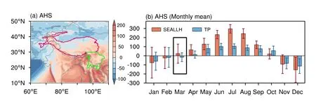
Fig.2.(a) Annual mean AHS (units: W m—2) and (b) long-term monthly means of the AHS (units: W m—2) averaged for the SEALLH and TP, along with their standard deviations.In (a), the region bounded by the green (red) solid line indicates the SEALLH (TP).

2.2.Atmospheric general circulation model

We adopted the atmospheric general circulation model ECHAM (version 6.3; ECHAM6) to confirm the excitation mechanism of the wave train by the Rossby wave source near northern Africa.The ECHAM6 was developed by the Max Planck Institute for Meteorology in Germany (Giorgetta et al., 2013; Stevens et al., 2013).Here, ECHAM6 was adopted with T63L47 resolution, corresponding to a horizontal resolution of about 1.875° and 47 vertical levels.The time step was set to 450 s following the default settings.

2.3.Statistical analysis and statistical tests

The statistical methods used in this paper include empirical orthogonal function (EOF) analysis without any rotation and regression analysis.The interdecadal component of a variable is extracted using a Lanczos low-pass filter with an 11-year cutoff period.The confidence levels of the linear regression and correlation are evaluated with a two-tailed Student’s t-test and using the effective degrees of freedom(Ndof), as defined by Bretherton et al.(1999):

whereNrepresents the sample size, andr1andr2are the lag-1 autocorrelations of the time series.The trends of all data are removed to avoid possible influences of global warming on the results.

2.4.Atmospheric heating source

The AHS is estimated using the hourly ERA5 data and the thermodynamic equations developed by (Yanai et al.,1992; Yanai and Li, 1994; Li and Yanai, 1996):

whereVis horizontal velocity (m s—1), θ is potential temperature (K), ω is vertical velocity at the isobaric surface (Pa s—1),∇is the isobaric gradient operator,tis time (s),pis pressure(hPa),Cp(1004 J kg—1K—1) is the specific heat at a constant pressure of dry air,p0= 1000 hPa, κ=R/Cp, andRis the gas constant of dry air (287.05 J kg—1K—1).In Eq.(2), ∂ θ/∂t,V·∇θ, ω(∂θ/∂p) reflect the contributions of the local tendency, the advection, and the vertical transfer to the apparent heat source.The column-integrated apparent heat source is calculated using Eq.(3):

In Eq.(3),pt= 100 hPa,psis the surface pressure (hPa),andgis the gravitational acceleration (m s—2).

2.5.Moist enthalpy

The enthalpy (hm; J kg—1) of moist air mass is calculated by the method of Neelin et al.(1987) and Neelin and Su(2005):

whereLv(2.5×106J kg—1) is the latent heat of vaporization for typical atmospheric temperatures,Tis the ambient temperature (K), andqis the mixing ratio (kg kg—1), i.e., higher moist enthalpy means higher temperature and humidity.

The column-integrated moist enthalpy flux is defined as:

whereV=(u,v) is the horizontal wind (m s—1),Vhmand∇·Vhmdenote the horizontal enthalpy transport (J m—1s—1)and its divergence (J m—2s—1), respectively (Wang et al.,2022).

2.6.Rossby wave source

The Rossby wave source (RWS; units: s—1) is calculated following Sardeshmukh and Hoskins (1988):

whereVχrepresents the horizontally divergent wind velocity(m s—1) and is defined as the gradient of velocity potentialχ(m2s—2).ζis the relative vorticity (s—1), andfis the Coriolis parameter.The RWS includes contributions from both the vortex stretching term and the advection of absolute vorticity by the divergent part of the flow (Sardeshmukh and Hoskins,1985; Mo and Rasmusson, 1993).

The anomalous RWS is computed following Watanabe(2004):

where the overbar and prime denote the climatological mean and monthly perturbation subtracted from the climatological mean, respectively.

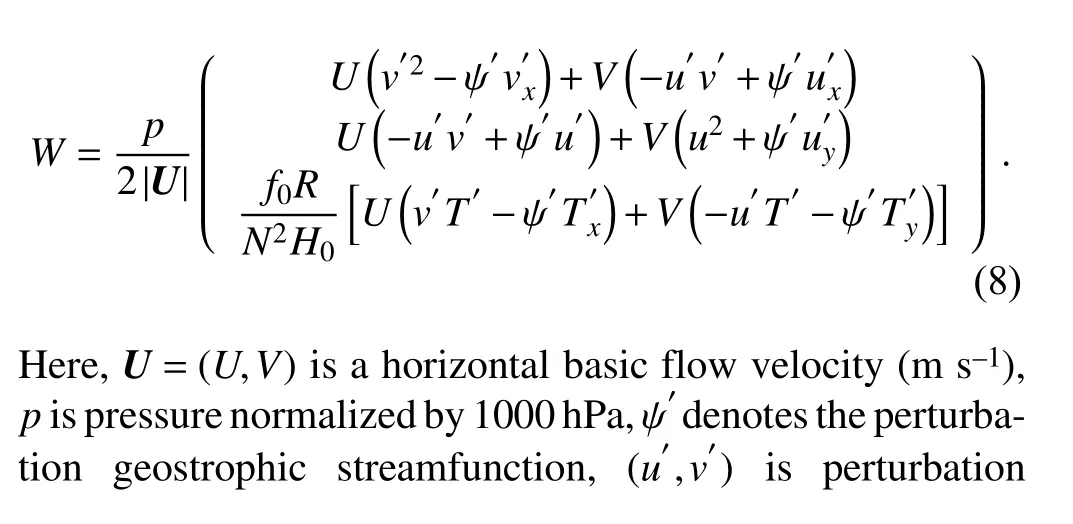
2.7.Wave-activity flux

The three-dimensional wave-activity flux was derived by Takaya and Nakamura (1997, 2001) based on the Plumb wave flux, making it more suitable for complex background airflow.The background field takes the average monthly climatological field for many years, which can better describe the energy dispersion characteristics of the stationary Rossby wave and the propagation anomaly of the Rossby wave.The three-dimensional expression of the wave-activity flux is as follows:

3.Interdecadal links between the March AHS in the SEALLH and CGT

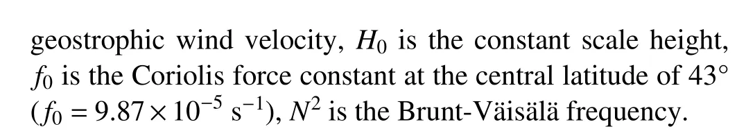
Figure 3 shows the spatial pattern of the first empirical orthogonal function (EOF1; Fig.3a) mode of the March AHS over the SEALLH and its normalized principal component time-series (PC1; i.e., the AHS index; Fig.3b).EOF1 is significantly separated from the remaining EOF modes(Fig.3c), based on the criteria of North et al.(1982), and has a monopole structure that explains 68.4% of the total variance of the March AHS in the SEALLH (Fig.3a).The positive phase of the EOF1 features a larger than average AHS over the entire SEALLH.The power spectra of the normalized AHS index time-series (Fig.3b) show a peak with an 8—11-year period (Fig.3d).Given that the peak passes a significance test at the 95% confidence level, a Lanczos low-pass filter with an 11-year cutoff period is applied to the AHS index to extract its interdecadal component (AHS-ID; Fig.3b).The AHS-ID explains 54.3% of the total variance of the AHS index, and is one of the most important components contributing to the variability of the March AHS in the SEALLH.

Following Branstator (2002), the EOF1 of the March 300-hPa non-divergent meridional wind is featured by a clear wave train-like structure with two negative centers over the Mediterranean and western India, and two positive centers over Somalia and the SEALLH in the upper troposphere (Fig.4a).We subsequently refer to the phase shown in Fig.4a as the positive phase of the CGT.The EOF1 is significantly separated from the remaining EOF modes and explains 27.0% of the total variance (Fig.4c).The PC1 time series of the March 300-hPa non-divergent meridional wind(i.e., the CGT index, Fig.4b) exhibits a significant interdecadal variation with a 10-year periodicity (Fig.4d).Consequently, a Lanczos low-pass filter with an 11-year cutoff period is also applied to the CGT index to extract its interdecadal component (CGT-ID; Fig.4b).The CGT-ID can explain 59.3% of the total variance of the CGT index, indicating that interdecadal variability is one of the most important components in the variability of the March CGT.

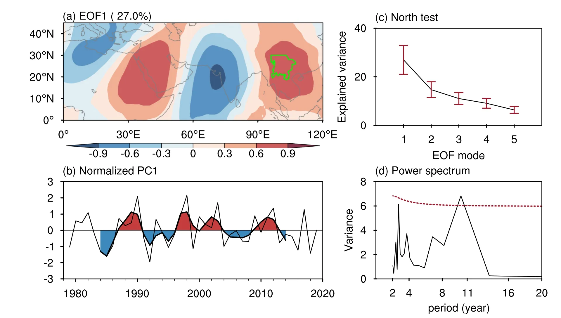
Fig.4.Same as in Fig.3, but for the 300-hPa non-divergent meridional wind (units: m s—1) of the region (0°—45°N,0°—120°E).

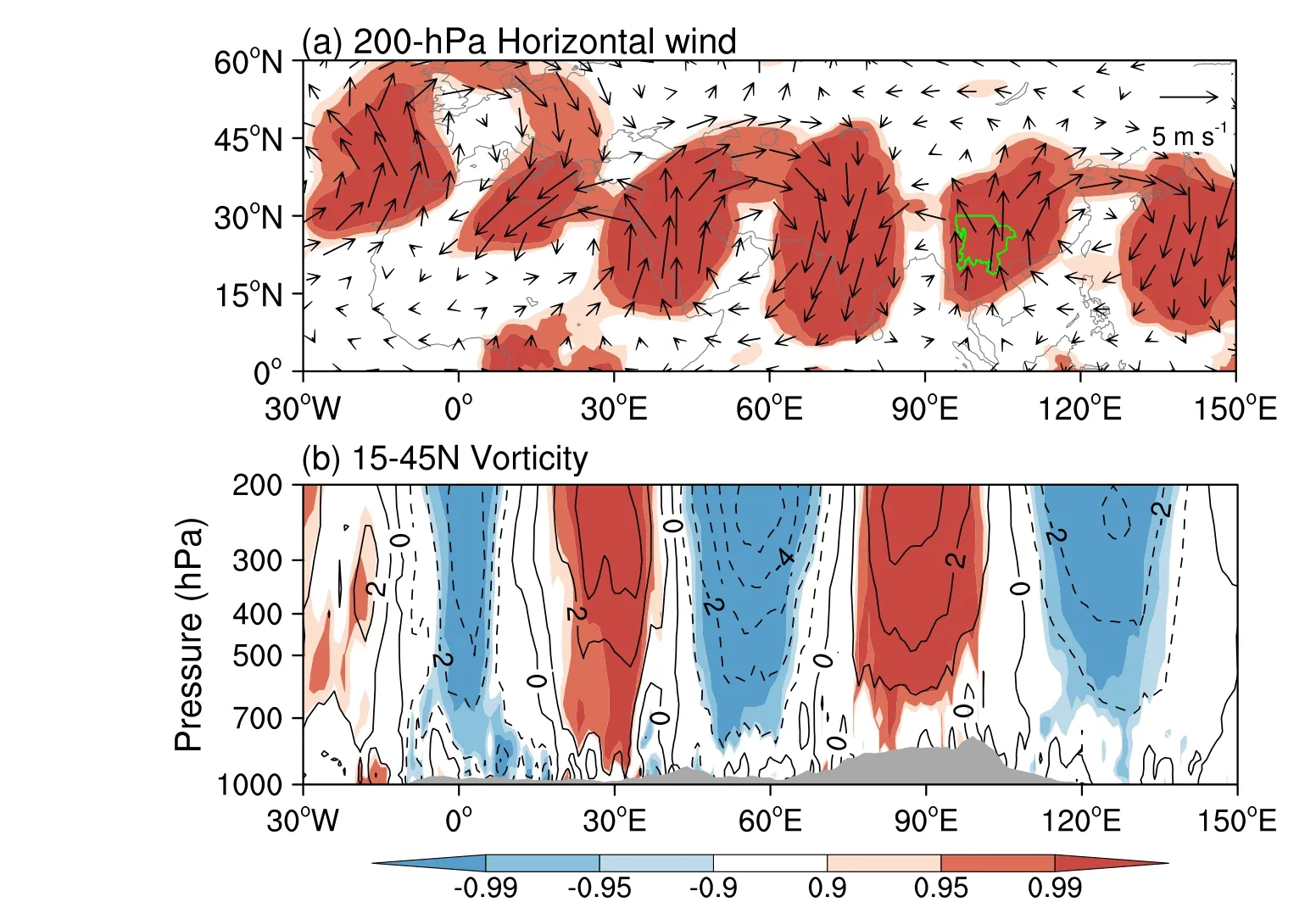
Fig.5.Composite differences of the March (a) 200-hPa horizontal winds (vectors;units: m s—1), and (b) 15°—45°N averaged relative vorticity (contour intervals: 10—6 s—1)between the positive phase of the CGT-ID and negative phase of the CGT-ID.In (a),the solid green line indicates the SEALLH.Light-to-dark shading indicates the 90%,95%, and 99% confidence levels based on a two-tailed Student’s t-test.

To delineate the structures and variations of the CGT on interdecadal time-scales, we further calculate the difference of associated variables using the CGT-ID averaged by 16 negative-phase years subtracted from the CGT-ID averaged by 15 positive-phase years (Fig.5).Figure 5a shows a clear wave train-like structure in the upper troposphere,with three anticyclonic centers over the Mediterranean, northwestern Indian subcontinent, and northwestern Pacific, and two anomalous cyclonic centers over northeastern Africa and the SEALLH.The wave train—like pattern presents an equivalent barotropic structure, with the maximum amplitude near the upper troposphere (Fig.5b).This difference shares the same structure as the CGT in boreal winter on the interannual timescale (Branstator, 2002).These results, confirming the result shown in Fig.4d, indicate that the March CGT undergoes interdecadal variations.

The correlation coefficient between the AHS-ID and CGT-ID is 0.96, which exceeds the 99% confidence level even after decreasing the effective degree of freedom to 12(Bretherton et al., 1999).This result suggests that the CGT is probably the driver of the March AHS variability over the SEALLH on an interdecadal timescale.To examine the pattern of the March AHS in the SEALLH and its link with the CGT, the March AHS data were regressed onto the CGT-ID for 1979—2019.It is clear that a wave train-like structure starts over Western Europe and passes through northeastern Africa and the Arabian Peninsula before finally reaching the SEALLH (Fig.6a).However, the anomalous central value of the AHS decreases to some extent.If we further divide the March AHS in the SEALLH into the column-integrated local tendency (CILT), column-integrated advection (CIA),and column-integrated vertical transfer (CIVT), these parameters can also be regressed onto the CGT-ID for 1979—2019.The regression of CILT onto the CGT-ID mostly differs from the CGT in terms of both its spatial structure and anomalous centers, indicating the CILT is not significantly related to the CGT on an interdecadal timescale (Fig.6b).The CIA regressed onto the CGT-ID, being most like the CGT(Figs.4a, 5), shows a positive CIA center with a maximum> 40 W m—2over the SEALLH (Fig.6c).Figure 6d also resembles the CGT (Figs.4a, 5).An anomalous center appears over the SEALLH with a maximum of > 25 W m—2.These results indicate that the CGT may affect the anomalous AHS by the advection and vertical transfer on an interdecadal timescale.

4.What physical processes link the March AHS in the SEALLH with the CGT on an interdecadal timescale?

4.1.Observational analysis

Figure 7a shows the 700-hPa horizontal wind anomalies regressed onto the CGT-ID.There are three anomalous anticyclonic centers over the Mediterranean, northwestern Indian subcontinent, and northwestern Pacific, and two anomalous cyclonic centers over northeastern Africa and the SEALLH.The 200-hPa horizontal wind anomalies regressed onto the CGT-ID (Fig.7b) exhibit a similar pattern to Fig.7a.The intensities of these anomalous anticyclones and anomalous cyclones gradually increase from the lower to upper troposphere, but their positions remain almost unchanged.Such a vertical distribution indicates that the interdecadal CGT is also a zonally oriented equivalent barotropic wave train resembling Fig.5.Because lines ABCDEFG (blue lines in Fig.7b)are mainly located in three anomalous anticyclonic centers and two anomalous cyclonic centers and traverse the SEALLH, the cross-section of anomalous vertical velocity is drawn along this line to illustrate the vertical transfer(Fig.7c).During the positive phase of the CGT, the significant ascending branches are mainly located around point B,between points C and D, and around point F, and the significant descending branches occur between point C, and between points D and E.The SEALLH is located in one of the significant ascending branches (around point F).To reveal more clearly how the anomalous AHS is induced, the column-integrated moist enthalpy flux and its divergence are further calculated (Fig.7d).It is clear that the air mass with higher moist enthalpy converges in the SEALLH(Figs.7a, b, d).Stronger than normal southerly winds are located on the eastern flank of the anomalous cyclone in the lower—upper troposphere, and an air mass of higher moist enthalpy converges and condenses over the SEALLH(Fig.7d), which results in a larger than average AHS over this region (Fig.6a).

The 200-hPa RWS is calculated to further determine the source of the CGT on an interdecadal timescale.The wave train structure is primarily excited by an anomalous RWS in the upper troposphere over northern Africa(Fig.8a; i.e., the Asian jet entrance indicated by the 40 m s-1contour of the climatological zonal wind) and propagates eastward to East Asia through the Arabian Peninsula, India, and the SEALLH.This is consistent with the disturbances near the core of the westerly jet that propagate eastward to the downstream area in a Rossby wave pattern because the jet acts as a waveguide (Branstator, 2002; Watanabe, 2004).Figure 8b shows that the 200-hPa wave-activity flux regressed onto the CGT-ID diverges from the positive RWS anomalies over northern Africa, crosses the negative RWS anomalies over the Arabian Peninsula, propagates eastward to the positive RWS anomalies over India, continues downstream and has negative RWS anomalies over the SEALLH, and then disperses in Japan.To address whether there is a decadal periodicity in the RWS over northern Africa, we calculate the 200-hPa RWS averaged over the rectangle in Fig.8a (20°—35°N,5°W—30°E) as the RWS index (Fig.8c).The RWS index has a strong interdecadal signal with a peak value around the 10-year band (Fig.8d).The correlation coefficient between the CGT-ID and the interdecadal component of the March RWS index is 0.83, which exceeds the 99% confidence level even after decreasing the effective degree of freedom to 11.These results confirm that the CGT affects the interdecadal variations of the March AHS over the SEALLH,which is mainly caused by the Rossby wave originating from northern Africa that propagates along the Asian jet stream in March.

4.2.Modeling results

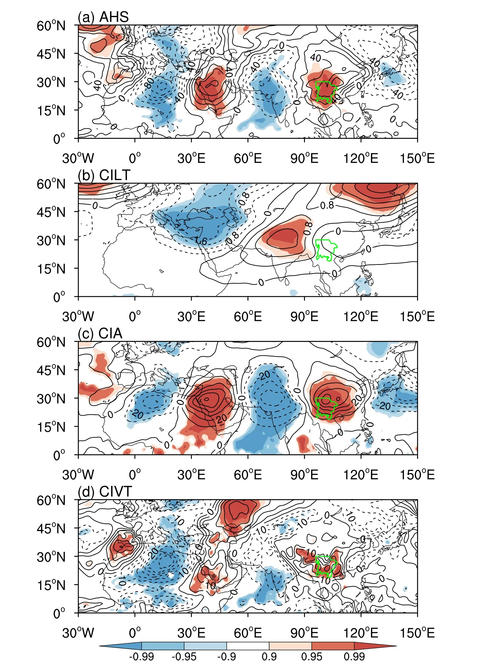
Fig.6.Regression of the (a) AHS (contour intervals: 20 W m—2), (b) columnintegrated local tendency (contour intervals: 0.4 W m—2), (c) column-integrated advection (contour intervals: 10 W m—2), and (d) column-integrated vertical transfer(contour intervals: 5 W m—2) onto the normalized CGT-ID in March during the period 1979—2019.Light-to-dark shading indicates the 90%, 95%, and 99% confidence levels based on a two-tailed Student’s t-test.The solid green line indicates the SEALLH.

Here, two sensitive experiments are conducted to confirm the possible mechanism of the CGT wave train modulated by the RWS over northern Africa.Sensitive experiment 1(SE1) is forced by the March RWS anomalies over northern Africa (20°—35°N, 5°W—30°E) regressed onto the CGT-ID in March (rectangle in Fig.8a).Sensitive experiment 2 (SE2)is forced by the same RWS but with opposite sign.In SE1 and SE2, the climatology RWS is used in other regions and other months except for northern Africa (20°—35°N, 5°W—30°E) and March.Other boundary conditions keep their climatological values.Each experiment is integrated for 20 years,and the first 5 years are discarded as the spin-up period.Analysis of the modeling results was performed over the last 15 years based on the differences between SE1 and SE2 (SE1 minus SE2).

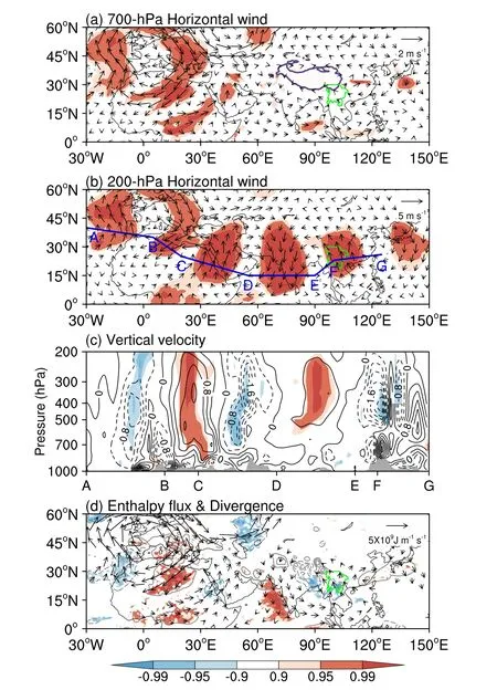
Fig.7.Regression of the (a) 700-hPa and (b) 200-hPa horizontal winds (vectors; units:m s-1), (c) vertical velocity (contour intervals: 4×10—3 Pa s—1) along line ABCDEFG shown in (b), and (d) column-integrated moist enthalpy flux (vectors; units: J m—1 s—1)and its divergence (contour intervals: 2×102 J m—2 s—1) onto the normalized CGT-ID in March during the period 1979—2019.In (b), the letters A (40°N, 30°W), B (35°N,5°E), C (25°N, 20°E), D (15°N, 55°E), E (15°N, 90°E), F (23°N, 100°E) and G (26°N,125°E) stand for the seven nodes on the CGT path (blue line).In (d), vectors exceeding the 95% confidence level are shown, and zero contours are omitted.Lightto-dark shading indicates the 90%, 95%, and 99% confidence levels based on the twotailed Student’s t-test.The solid green line indicates the SEALLH.

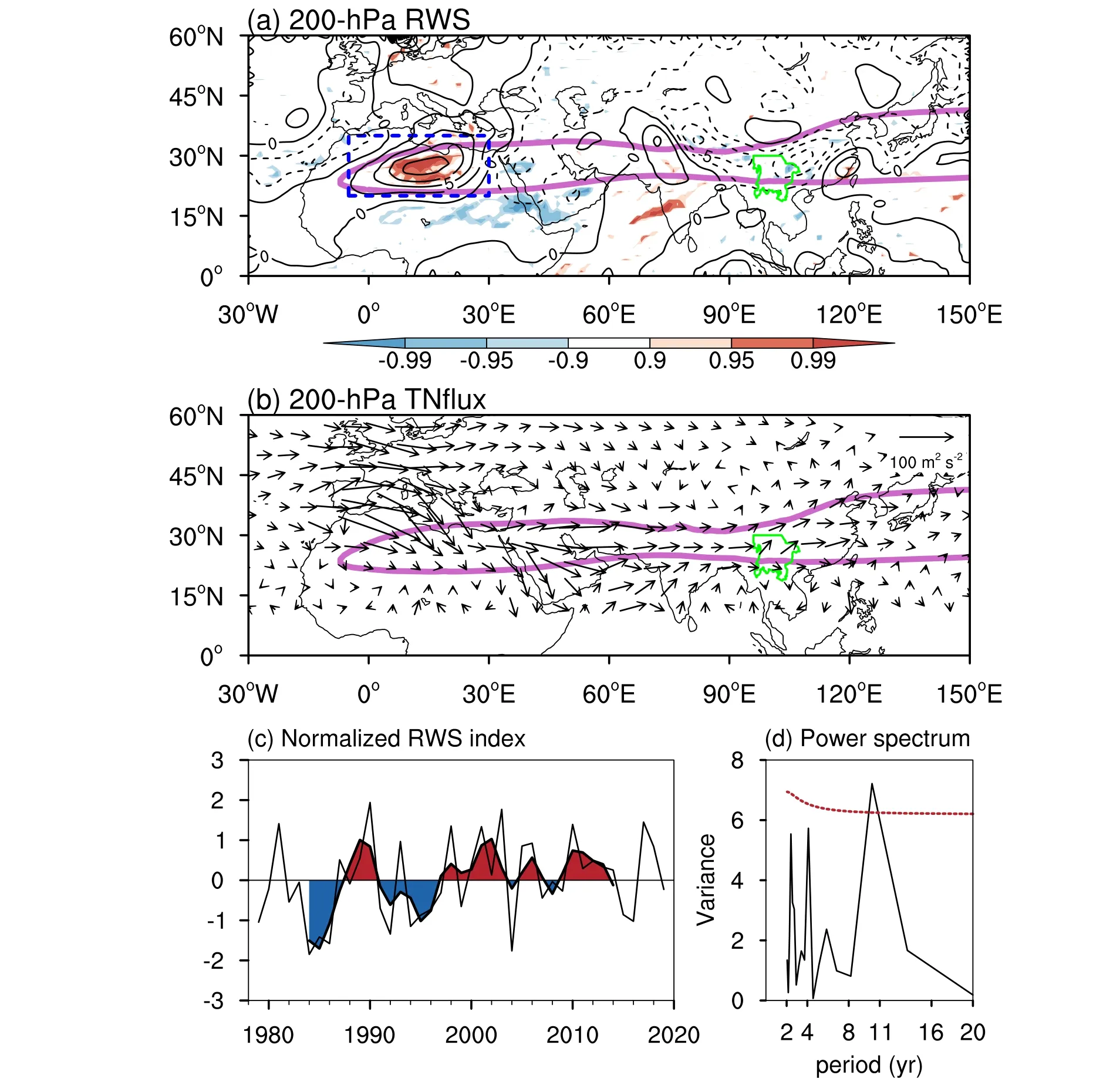
Fig.8.Regression of the 200-hPa (a) RWS (contour intervals: 2.5 × 10—11 s—2) and (b) waveactivity flux (m2 s-2) onto the normalized CGT-ID in March during 1979—2019.(c) Time series of the RWS index (thin line) and its interdecadal component (thick line with infilled colors).(d) Power spectral density of the RWS index.In (a), the light-to-dark shading indicates the 90%, 95%, and 99% confidence levels based on the two-tailed Student’s t-test.In (a) and (b), the solid purple line indicates the 40 m s—1 contour of climatological zonal wind.The solid green line indicates the SEALLH.In (d), the red line shows the 95%confidence level of the corresponding red spectrum.

We analyzed simulated differences in the 200-hPa horizontal winds, 15°—45°N averaged relative vorticity, columnintegrated moist enthalpy flux, and its divergence in March.The simulated differences of the 200-hPa horizontal winds almost share the same pattern as the diagnostic results for the research domain (Figs.5a and 9a), although the centers of the anomalous anticyclones around the Mediterranean and near northern Africa somewhat differ from the observational analysis.Two anomalous anticyclonic centers over the northwestern Indian subcontinent and northwestern Pacific, and one anomalous cyclonic center over the SEALLH, perfectly match the observational results.The wave train—like structure also presents an equivalent barotropic structure, with the maximum amplitude near the upper troposphere (Fig.9b).The relative vorticity in the regions west of North Africa shows an opposite distribution to Fig.5b, suggesting that the cyclonic RWS anomalies over northern Africa only propagate downstream along the westerly jet.These results confirm the major role of the RWS over northern Africa in driving the phase of the CGT on an interdecadal timescale.The anomalous southerly column-integrated moist enthalpy flux is well reproduced in the SEALLH (Fig.9c).The higher moist enthalpy air mass converges over the SEALLH, leading to an increase in the AHS in the SEALLH.The simulated results obtained above confirm that the RWS over northern Africa forcing the CGT plays a significant role in regulating the interdecadal variation in AHS over the SEALLH.

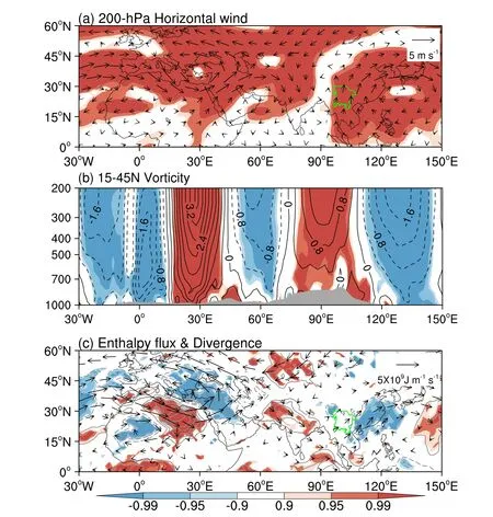
Fig.9.Composite differences of the March (a) 200-hPa horizontal winds (vectors; units:m s—1), (b) 15°—45°N averaged relative vorticity (contour intervals: 10—6 s—1), and (c) columnintegrated moist enthalpy flux (vectors; units: J m—1 s—1) and its divergence (contour intervals:2×102 J m—2 s—1) between SE1 and SE2.In (a), the solid green line indicates the SEALLH.Light-to-dark shading indicates the 90%, 95%, and 99% confidence levels based on a twotailed Student’s t-test.

5.Summary and discussion

This study has investigated the interdecadal variations of the March AHS over the SEALLH and its possible causes based on the fifth-generation reanalysis dataset from the European Centre for Medium-Range Weather Forecasts for the period 1979—2019.The positive EOF1 phase of the March AHS over the SEALLH is characterized by a monopole structure with a larger-than-average AHS over the entire SEALLH.The interdecadal component of the AHS index explains 54.3% of the total variance, highlighting its importance in controlling the variability of the March AHS over the SEALLH.The March CGT is characterized by an equivalent barotropic wave train along the Asian westerly jet stream in the upper troposphere, which also has a significant interdecadal variation that explains 59.3% of the total variance.

The interdecadal variation of the March AHS over the SEALLH is significantly related to the CGT on the same timescale.When the CGT is optimally excited by the significant vorticity source near northern Africa in its positive phase, the SEALLH is dominated by anomalous southerly winds and ascending motions.The enhanced southerly winds and upward motions located on the region east of the anomalous cyclone, further transport a higher moist enthalpy air mass into the SEALLH, which converges and condenses, ultimately resulting in a larger than average March AHS over this region.When the CGT is in its negative phase, the opposite condition can be observed to a large degree.The simulated results confirm the impact of the RWS over northern Africa on the interdecadal variation of the AHS over the SEALLH through its phase modulation of the CGT.This key physical process links the March AHS over the SEALLH with the CGT on an interdecadal timescale, as is schematically shown in Fig.10.

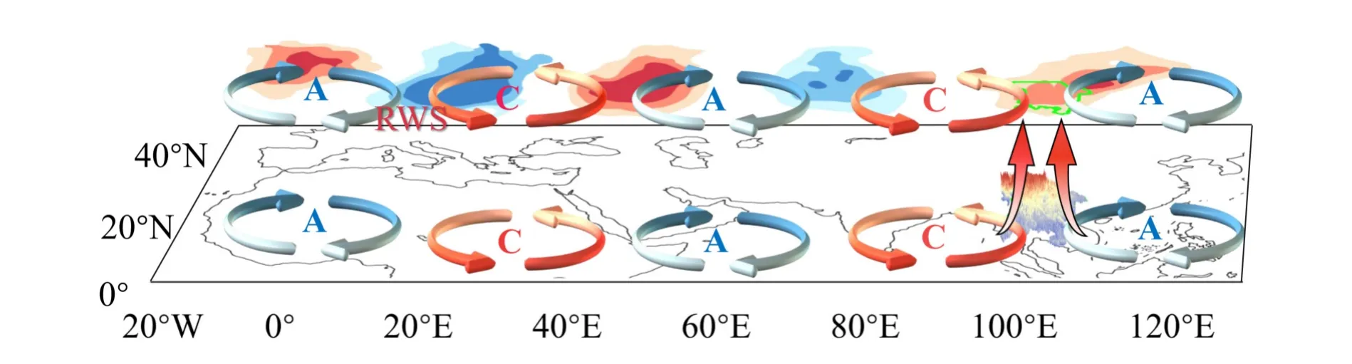
Fig.10.A schematic diagram of the effects of the CGT on atmospheric heat sources in the SEALLH.The letters A and C denote an anomalous anticyclone and cyclone, respectively.

The Atlantic Multidecadal Oscillation (AMO;Schlesinger and Ramankutty, 1994) and Pacific Decadal Oscillation (PDO; Mantua et al., 1997) are two significant signals on the interdecadal timescale.The correlation coefficient between the AHS-ID and the interdecadal component of the March AMO index is 0.36.The correlation coefficient between the AHS-ID and the interdecadal component of the March PDO index is —0.26.These two correlation coefficients are insignificant, even at the 90% confidence level.Apparently, the AMO and PDO are not the main factors that directly influence the interdecadal variations of the AHS over the SEALLH on interdecadal timescales.

Previous studies have pointed out that the AHS and surface heat flux over the anomalous centers of the CGT contribute somewhat to the formation and variability of the CGT (Enomoto, 2004; Yasui and Watanabe, 2010; Chen and Huang, 2012; Lee et al., 2017; Yang et al., 2021).In this study (Figs.8a, b), we found a significant relationship between the RWS over northern Africa and the CGT-ID.All results imply that an interaction exists between the CGT and AHS located around the anomalous centers of the CGT.The relative contributions of the CGT and associated AHS to the interaction is beyond the scope of this study.In subsequent studies, we intend to clarify the physical processes involved in the interaction between the RWS in northern Africa and CGT through numerical experiments.

Acknowledgements.This work was supported by the National Natural Science Foundation of China (Grant No.42030603), the Natural Science Foundation of Yunnan Province(2019FY003006), and the Postgraduate Research and Innovation foundation of Yunnan University (2021Z017).