Jianling Wang ,Zihuang Cao ,Yang Huang ,and Haibo Yuan

1 CAS Key Laboratory of Optical Astronomy,National Astronomical Observatories,Beijing 100101,China;wjianl@bao.ac.cn

2 Department of Astronomy,Beijing Normal University,Beijing 100875,China

Abstract Large scale spectroscopic surveys such as that using Large-sky Area Multi-Object Fiber Spectroscopic Telescope(LAMOST)have collected spectra of millions stars in the Milky Way.Utilizing this huge sample of stars to study the assembling history and structure of our Galaxy requires accurate estimates of distance,extinction,age,and mass for individual stars.Combining the parallax constraint from Gaia EDR3 with Bayesian inference,we have estimated the distance and extinction for stars observed in LAMOST DR7,as well as the stellar mass and age for evolved stars in this data release.We validated the accuracies of the stellar parameters by comparing our results against various measurements,including the star-pair technique,asteroseismology,globular clusters,and isochrone fits to main sequence stars and subgiants.This is a valuable catalog of stellar parameters under a Bayesian framework estimated using the data from Gaia EDR3 and LAMOST spectroscopic data.With this data set we explored the stellar population of the Galactic massive substructure Gaia-Sausage-Enceladus (GSE).The kinematically selected members of GSE have a median metallicity of [Fe/H]=−1.29 and a median age of 11.6 Gyr.

Key words: stars:distances–stars:fundamental parameters–stars:kinematics and dynamics–Galaxy:formation– (Galaxy:) globular clusters: general

1.Introduction

We have entered a golden era of Galactic archaeology with many large-scale sky surveys and huge data sets available in both photometry and spectroscopy,e.g.,the Two Micron All-Sky Survey (2MASS,Skrutskie et al.2006),the Sloan Digital Sky Survey (SDSS,York et al.2000),the Sloan Extension for Galactic Understanding and Exploration(SEGUE,Yanny et al.2009),the Large-sky Area Multi-Object Fiber Spectroscopic Telescope (LAMOST,Deng et al.2012;Liu et al.2014),the Apache Point Observatory Galactic Evolution Experiment(APOGEE;Majewski et al.2017),and the Gaia mission (Gaia Collaboration et al.2016,2018,2021).These ambitious surveys have provided valuable information for a large number of stars,and are essential for understanding the structure,formation,and evolution of our Galaxy.It is expected that in the next decade the ongoing (e.g.,LAMOST and Gaia) and upcoming(e.g.,4MOST,WEAVE;Dalton et al.2014;de Jong et al.2019) surveys will continually revolutionize our view on the Galactic structure and its assembling history.

To make full use of these surveys to study the assembling history of our Milky Way,it is crucial to derive and use the multi-dimensional information on individual stars.These astrophysical properties include the six-dimensional phase space coordinates(i.e.,three-dimensional(3D)position and 3D velocity),metallicity and chemical abundances,photometries,age,and extinction.The combination of these astrophysical parameters can be used to reconstruct the assembly history of the Galaxy.Chemo-dynamical studies have led to many new findings,such as stellar streams,dwarf satellites,and clumps.One of the major contributions of Gaia to this field is the discovery of the so-called Gaia-Sausage-Enceladus (GSE;Belokurov et al.2018;Helmi et al.2018;Xiang &Rix 2022),a major merger event of the Milky Way 8–11 Gyr in age.Now our inner halo is almost dominated by the relics of this massive merger event.This finding is achieved by the analysis of kinematics,chemistry,age,and spatial distribution of stars,which demonstrate the importance of the combination of multi-dimensional information on individual stars.

The LAMOST Galactic survey began its regular survey in the fall of 2012,which was the first spectroscopic survey to obtain spectra of over 10 million stars,and regularly released basic stellar parameters measured with the official LAMOST stellar parameter pipeline (LASP;Wu et al.2011;Luo et al.2015).These stellar parameters include effective temperatureTeff,metallicity [Fe/H],surface gravitylogg,and the line-ofsight velocityVr.To fully make use of this huge data set for Galactic archaeology,it is of vital importance to provide an estimate of distance,extinction,age,and stellar mass.In addition to those basic stellar parameters,in the Value-Added Catalog,more physical parameters (like the distance,extinction,mass,and age) from the LAMOST surveys are provided to the community(e.g.,Wang et al.2016b;Xiang et al.2017a).For example,using the isochrone fitting method,Xiang et al.(2017b) derived stellar ages for around 1 million main sequence turnoff stars and subgiants in the LAMOST Spectroscopic Survey of the Galactic Anti-center (LSS-GAC;Liu et al.2014).Xiang &Rix (2022) derived ages for subgiants in LAMOST Data Release 7 (DR7) with the Bayesian isochrone fitting method.Huang et al.(2020)derived distances,masses,and ages for ∼140,000 primary red clump stars with a kernel principal component analysis method.The measurements of the previous studies were usually based on different methods,different models,and different prior functions,which usually caused systematic errors (Pinsonneault et al.2018).It would be useful to check those results from different approaches.

It has been demonstrated that Bayesian inference is a powerful and important method in astrophysics,especially in deriving stellar parameters (Burnett &Binney 2010;Burnett et al.2011;Binney et al.2014;McMillan et al.2018;Queiroz et al.2018;Aguirre Børsen-Koch et al.2022;Anders et al.2022;Wang et al.2022b).With this approach,we have derived distance and extinction for the LAMOST spectroscopy survey (Wang et al.2016b)and SDSS/APOGEE survey(Wang et al.2016a).In the current work,we improved our former calculation by imposing constraints with parallaxes from Gaia Early Data Release 3(EDR3).With extensive comparisons with independent measurements,we show that accurate parallaxes are important for obtaining accurate stellar parameters,especially for significantly improving the accuracies of stellar ages and masses.

The paper is structured as follows.In Section 2,we briefly describe the methodology and data employed in the current analysis.In Section 3,we compare our estimates of distance,extinction,mass,and age with independent measurements in the literature.In Section 4,we use these data to study the age and metallicity of GSE substructures.Finally,a summary is given in Section 5.

2.Methodology and Data

In Wang et al.(2016a,2016b),we applied the Bayesian method to estimate the distance and extinction to stars observed by both the LAMOST and APOGEE surveys.The observables used in this method include stellar parametersTeff,logg,and[Fe/H],from LAMOST/APOGEE spectra,and infrared photometriesJ,H,Ksfrom the 2MASS survey.In this work,we include the constraint of Gaia parallax (ϖ).These observables form an observed vector

Each star can be characterized by a set of “intrinsic”parameters: metallicity [M/H],age τ,initial mass M,position on the skyl,b,and distance from the Sund.These quantities also form another vector

With trivial Bayesian theory,we can determine the posterior probability of P(X|O),which is the conditional probability of the parameter set X given O

whereP(O|X)is the likelihood of O given the parameter set X.O and X can be connected by theoretical isochrones.P(X)is the prior probability ascribed to the set of parameters.A Gaussian function is used to associate the measured observables for each component of O with a meanand standard deviation.

An extinction model and a three-component model of the Galaxy for the distribution functions of metallicity,density,and age are used for the prior probability,P(X)

Herei=1,2,3 correspond to thin-and thick-disk,and stellar halo,respectively.

The extinction prior model (AVprior(ℓ,b,d)) is taken from Sharma et al.(2011) with normalization to infinity adopted from Schlegel et al.(1998).The Padova stellar isochrones3http://stev.oapd.inaf.it/cgi-bin/cmdare used.With the posterior distribution function P(X|O)in hand,it is trivial to derive the moments for each componentxiof X.The first and second moments for each componentxiof X are the expectation and uncertainties for each stellar parameter respectively.In the current work,we derived the expectation values and their associated uncertainties for four stellar parameters: stellar distance,extinction,stellar mass,and age.For details on the method,please refer to Wang et al.(2016a,2016b),Burnett &Binney (2010),Burnett et al.(2011),Binney et al.(2014).

In the current work,we follow the same method as used in Wang et al.(2016a,2016b),but with several improvements.First,the metallicity resolution of isochrones is increased to a step of 0.05 dex ranging from −2.2 to 0.5.These improved resolutions in metallicity result in 55 metallicity isochrones,which are a factor of 2.5 larger than those used in Wang et al.(2016a,2016b).Even though the uncertainty of observed stellar metallicity is larger than this value,higher resolution of metallicity in isochrones helps break the degeneracy between metallicity and age for the internal precision,especially for the stellar age.We note that this metallicity bin size is within the ranges of the literature using a Bayesian framework for stellar parameter estimation.Sanders &Das (2018) relied on a bin size of 0.01 dex in metallicity following similar methodology as us for stellar age estimation,but considering Gaia Data Release 2(DR2)parallax.Anders et al.(2022)used 0.1 dex in metallicity bin size in their “StarHorse”code.Lin et al.(2022)adopted 0.04 and 0.03 dex bin sizes for metallicity in the range[−3,−1] and [−1,0.5],respectively.Second,we imposed parallax constraints from Gaia EDR3(Gaia Collaboration et al.2021) in the observable vector O,the errors of which are considered in Equation (4).We note that the systematic errors in the Gaia EDR3 parallaxes were corrected following the method suggested by Lindegren et al.(2021),which are also validated by independent checks(Huang et al.2021;Zinn 2021;Wang et al.2022a).These improvements lead to accurate estimates of stellar parameters as demonstrated in the following sections.

In this work,we utilize LAMOST DR7 with atmospheric parameter measurements for around 5 million stars (Wu et al.2011;Luo et al.2015).We cross-matched this catalog with Gaia EDR3 to obtain parallax.There are 204,878 stars without parallaxes available in Gaia EDR3,for which we set their parallax errors to infinite.This corresponds to a flat prior in the parallax constraint.In Appendix A,we discuss the uncertainties of distance,extinction,stellar mass,and age yielded by our method.

3.Comparison and Validation with External Measurements

In this section we compare the distance,extinction,mass,and age for stars measured with our Bayesian inference to those in the literature.In this way,we have an overview on the accuracy and any systematic uncertainties of our measurements.In the following comparisons,we will select LAMOST data with signal-to-noise ratio (S/N) greater than 20 unless otherwise stated.

3.1.The Distance

The left panel of Figure 1 compares the distance derived by our Bayesian method with LAMOST data with that derived with Gaia EDR3 parallaxes.In this comparison,10%uncertainties of Gaia EDR3 parallax data are selected for cross-matching with LAMOST data.The red crosses indicate the median values,and the error bars show the 1σ dispersion in each bin.Thanks to the constraints from the Gaia EDR3 parallax used in our Bayesian method,the distance derived is well correlated with the distance of Gaia EDR3 with tiny uncertainties.There are many stars with large deviation from the one-to-one straight line.There could be several reasons for these stars,e.g.,large uncertainties in stellar atmospheric parameters from spectroscopic observation,and the mismatch of stars between LAMOST data and Gaia EDR3 due to large proper motion (PM).

Figure 1.(Left) Comparing distance derived by our Bayesian method with that of Gaia EDR3 parallax.The black-dashed line shows the one-to-one line.The red crosses indicate the median values,and the error bars show the 1σ dispersion.The color bar on the right indicates the number density.(Right)The fractional difference distribution of parallax.The values of median and dispersion are labeled on the top left.In the comparison with Gaia EDR3 data,the criterion of σϖ/ϖ<0.1 has been used to select parallax with high accuracy.

The right panel of Figure 1 displays the distribution of fractional difference in the parallaxes between our measurement and Gaia EDR3,where the values of mean and dispersion are labeled on the top left.There are large extended wings in the distribution of fractional difference of parallaxes,which are linked to the stars with large deviation from the one-to-one correspondences in the left panel of Figure 1.Several reasons may cause this.

Figure 2.Comparing the extinction Av derived by our Bayesian method with that from the star-pair method(Yuan et al.2013).The left panel shows results of giants withlogg <3.5,and the right panel exhibits dwarf stars withlogg >3.5.The median difference and 1σ dispersion are labeled on the top left of each panel.The bluedashed line in each panel indicates the one-to-one correspondence.The background gray-scale image in each panel signifies the number density of stars.

3.2.The Extinction

In this section we compare the extinction measured by our Bayesian method with measurement with the star-pair technique (Yuan et al.2013).This technique has been applied to LAMOST data to estimate the extinction of individual stars,which is provided in the Value-Added Catalog of the LAMOST survey (e.g.,Xiang et al.2017b).In our method,we used the Cardelli et al.(1989) extinction curve withRV=3.1 to calculate the extinction of theKsband(AKs),which provides a relationAKs=0.117Av(for details please refer to Wang et al.2016b).With the star-pair technique,Yuan et al.(2013) suggest the extinction coefficient ofR(Ks)=0.306.To make a fair comparison,we used the same extinction curve(Cardelli et al.1989) to convert theirAKstoAv.

Figure 2 features the comparison ofAvbetween our extinction and that derived by the star-pair method in the LAMOST Value-Added Catalog DR2 (Xiang et al.2017b),separated into giant (logg<3.5,left panel) and dwarf (logg>3.5,right panel)stars.The median difference ofAvderived from the two independent methods is very small,i.e.,0.01 and 0.03 mag for giants and dwarfs,respectively,with a dispersion of ∼0.2 mag.

3.3.The Stellar Mass

In this section,we compare the stellar mass to other measurements.We note that it is only possible for mass and age estimation for evolved stars,since the identification of mass and age using theoretical isochrones is very difficult for main sequence stars.We will hereafter consider evolved stars with logg<3.9 for their mass and age validation in this section and the following section.

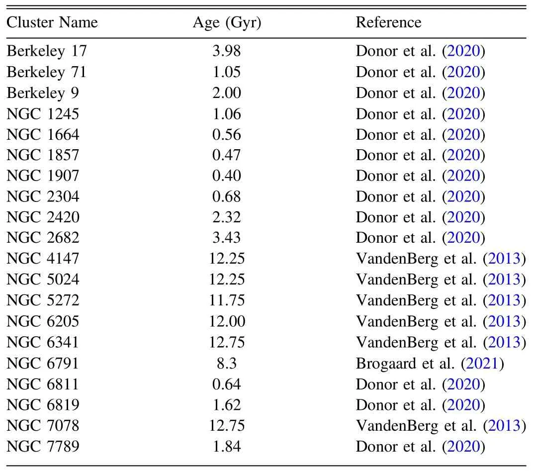
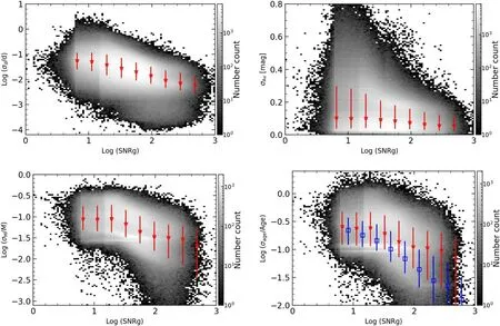
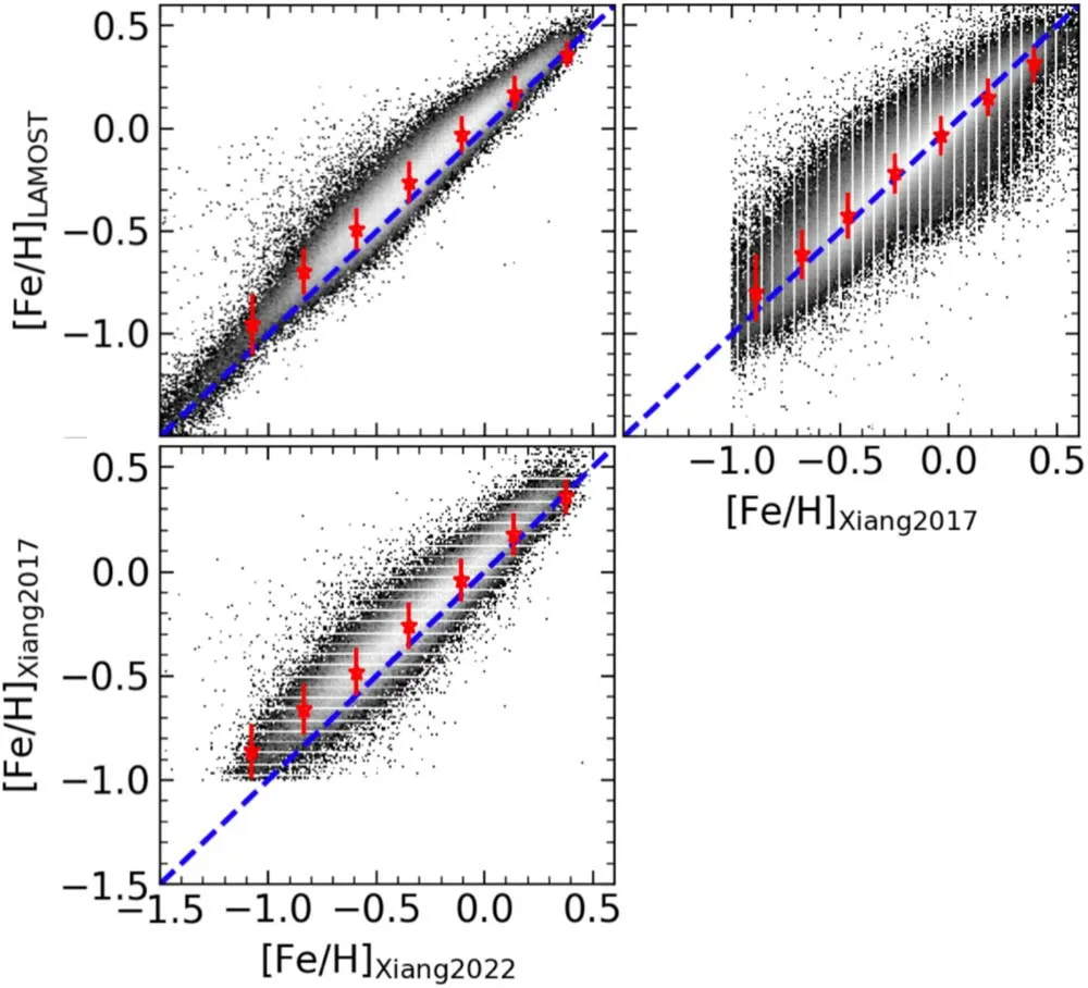
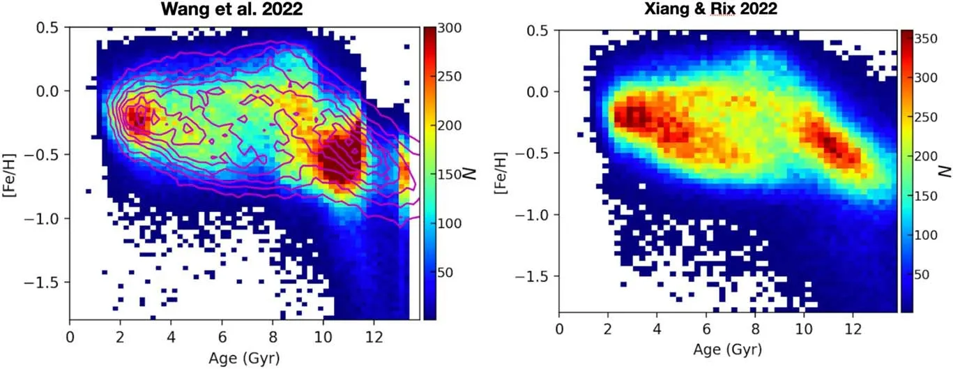
Pinsonneault et al.(2018)derived masses and ages for 6676 evolved stars (1

Figure 3 compares our Bayesian stellar mass to that derived by Pinsonneault et al.(2018).There is good agreement between the stellar mass estimated by these two independent measurements,while there is a general trend that at high mass theMKeplertends to be larger.The mean difference for the whole sample is 0.06M⊙,with a dispersion of 0.23M⊙.The median value and 68 percentile interval of fractional difference are

Xiang et al.(2017a) estimated stellar age and mass for ∼1 million main sequence turnoff and subgiant stars from the LAMOST spectroscopic survey.They also adopted a Bayesian algorithm with observation data derived from LAMOST spectra,includingTeff,absolute magnitudeMv,[Fe/H],and[α/ Fe].Even though they adopted the Bayesian algorithm as we did,there are great differences,e.g.,the prior function,isochrone models,and,more importantly,constraints given by Gaia parallax.Therefore,it is interesting to compare the results from these two methods.Figure 4 compares the estimated stellar masses,which show good correlation.The red stars indicate the median value at each bin,which shows that the mass from Xiang et al.(2017a) is slightly larger than ours at large mass range.The median difference is only 0.05M⊙,and dispersion is 0.12M⊙.The median value of fractional difference is 0.04,and the 68 percentile interval of the fractional difference is [−0.11,0.05].

Figure 3.Comparing stellar mass estimated by our Bayesian method to that derived with asteroseismic data for giant stars (Pinsonneault et al.2018).The red stars indicate the median value for each bin,and error bars signify the dispersion in each bin.The blue-dashed line indicates one-to-one correspondence.The median value and 68 percentile interval of fractional difference distribution are labeled on the top left with red color.

Figure 4.Comparing stellar mass estimated with our Bayesian method to that from Xiang et al.(2017a) for main sequence turnoff stars and subgiants.The spectral data with S/N>20 were used in this comparison.The blue dashed line indicates the one-to-one correspondence.The median value and 68 percentile interval of fractional difference distribution are labeled on the top left with red color.

Figure 5.Comparing stellar age measured in current work for giant stars to that from Pinsonneault et al.(2018) with asteroseismic data.The blue-dashed line indicates the one-to-one correspondence,and the red stars and error bars show the median value and 1σ dispersion in each bin respectively.The red numbers on the top left express the median value and 68 percentile interval of fractional difference distribution.

Figure 6.Comparing the stellar age for main sequence turnoff stars and subgiants in the current work to that from Xiang et al.(2017a).The bluedashed line shows the one-to-one correspondence,and red stars and error bars indicate the median and dispersion in each bin respectively.The median value and 68 percentile interval of fractional difference distribution are labeled on the top left with red color.

Figure 7.Comparing the stellar age for subgiant samples in the current work to that from Xiang &Rix (2022).The blue-dashed line indicates the one-to-one correspondence.The red stars and error bars signify the median and dispersion in each bin.The median value and 68 percentile interval of the fractional difference distribution are labeled on the top left.

3.4.The Age

In this section,we compare our stellar age to those estimated from other independent methods.As noted in the above section,only evolved stars withlogg<3.9 are considered in this section.

The asteroseismic data are powerful for constraining stellar mass,and then stellar age.Figure 5 compares stellar age estimated with asteroseismic data for giant stars from Pinsonneault et al.(2018).The stellar ages estimated with these two different methods are consistent with each other,while the ages from Pinsonneault et al.(2018) are larger than ours when ages are greater than 5 Gyr.The median value of fractional difference is 13%.

Figure 8.Comparing individual star ages of cluster members measured in the current work to the age of clusters in the literatures.The blue-dashed line indicates the one-to-one correspondence.The red stars and error bars signify the median value and dispersion in each bin respectively.The median value and 68 percentile interval of the fractional difference distribution are labeled on the top left.

The ages of main sequence turnoff stars and subgiants can be relatively accurately estimated,since in these evolution stages,the atmospheric parameters of these stars vary significantly with age.However,for the main sequence stars it is difficult to estimate their ages as the isochrones of different ages are tightly crowded together (Xiang et al.2017a).Xiang et al.(2017a)measured the ages for ∼1 million stars’main sequence turnoff and subgiant stars selected from the Value-Added Catalog of the LAMOST Galactic survey (Xiang et al.2017b).Figure 6 compares our stellar ages to those in Xiang et al.(2017a).The stellar ages are correlated well,while there is systematic offset for age larger than 4 Gyr.We discuss this large systematic offset in Appendix B.We note there is a cutoff of age at∼13.2 Gyr in our age estimation,which results from an imposed limitation by the Padova isochrones.

Recently,Xiang&Rix(2022)applied a Bayesian method on LAMOST DR7 to derive stellar age for subgiant stars.There are several differences between theirs and ours.First,the input parameters are different.They usedMK,Teff,[Fe/H],and [α/Fe],Gaia parallax,and Gaia and 2MASS photometries.We note that stellar labels used in their method are derived from the data-driven Payne (DD-Payne) approach,while what we used are from the LAMOST pipeline LASP (Wu et al.2011;Luo et al.2015).Second,they adoptedYYstellar isochrones,while the Padova isochrones are utilized in our method.Third,the extinction estimation is different.They estimated the extinction with a methodology of the intrinsic colors empirically inferred from their stellar parameters,while our extinction is calculated self-consistently in the Bayesian inference.Figure 7 compares the stellar ages estimated in the current work to those from Xiang&Rix(2022).Even though there are many differences in deriving the stellar age,both methods produce a well correlated stellar age.This may reflect the facts that the age of subgiant stars is well determined with high precision,and that the constraints from Gaia parallax are important for retrieving accurate age.We note there is only a 0.11 Gyr systematic offset in this comparison,with fractional difference beingIn Figure C1 we also check the relation between stellar age and metallicity for comparison with Xiang &Rix (2022).

Figure 9.The kinematic distribution of stars.GSE stars are selected following Feuillet et al.(2021)labeled by red points.The black density shows our main samples.For details on the sample selection please refer to the text.

Figure 10.(Bottom left) Age–metallicity relation for giant stars with log g<3.9.The GSE stars selected following Feuillet et al.(2021) are displayed with red points.(Top) Age distribution for GSE stars.(Right) Metallicity distribution of GSE stars.

Star members for a star cluster are believed to form from a single molecular cloud at the same time.Therefore,the star members share a single age which is the cluster age.A star cluster provides unique opportunities to test the age accuracies of stellar age estimates.In this section,we compare individual stellar ages to cluster ages from the literature.

In order to identify the member stars for a given cluster,we use two well studied star cluster catalogs in which star members for each cluster have been carefully identified.One is from Mészáros et al.(2013),which provide 20 star clusters including both open and globular clusters.These clusters served as calibration to the pipeline of APOGEE in Sloan Digital Sky Survey-III (SDSS-III).The other is the Open Cluster Chemical Abundances and Mapping survey from Donor et al.(2020),which provides large uniform,infraredbased spectroscopic data for 128 open clusters to constrain the key Galactic dynamical and chemical evolution parameters.The cluster member stars have been selected based on stellar radial velocities,PMs,spatial location,and derived metallicity as membership discriminators.A visual inspection by several authors for each cluster is performed to guarantee the quality of member selection.

We cross-matched these two star cluster catalogs with LAMOST DR7 entries,and selected cluster member stars with logg<3.9.Finally,we obtain 79 members belonging to 20 clusters.In Table 1 we list the clusters used in the current work and the age adopted for each cluster and their references.For the open clusters,the ages are adopted from Donor et al.(2020),while for the globular clusters their ages are taken from VandenBerg et al.(2013).One special case is the open cluster NGC 6791.The age of this old super-metal-rich([Fe/H]=0.4)open cluster has been studied by Grundahl et al.(2008) from comparisons with theoretical isochrones in the mass–radius diagram.They found the cluster is old with age from 7.7 to 9.0 Gyr,depending on the adopted models.This age is consistent with the estimate from the eclipsing binary method from Brogaard et al.(2021),8.3±0.3 Gyr.Therefore,8.3 Gyr is adopted in our analysis.

Table 1 Age and Reference for the Star Clusters Used in the Current Work

Figure 8 compares individual star ages measured by our Bayesian method to the cluster age.Both ages agree well generally,even though there are some stars with large deviations from the one-to-one correspondence line.There are two clusters with large age deviations from our estimate,which are NGC 2420 and NGC 2682.We note the age of open cluster NGC 2682 is 3.43 Gyr estimated by Kharchenko et al.(2013) with stellar data from PPMXL and 2MASS.Based on Gaia DR2 its age is estimated to be 3.64 Gyr by Bossini et al.(2019) and 4.3 Gyr by Cantat-Gaudin et al.(2020).The new results based on Gaia data lead this cluster age to be closer to our estimation,∼4.0 Gyr.

4.The GSE Substructure in LAMOST Survey

In the above section we have extensively compared the distance,extinction,mass,and age,measured with our Bayesian method to those derived with completely independent methods.These comparisons validate our results.These data will be valuable for studies on Galactic structure,formation,and evolution.Below we use these data to explore the properties of the Galactic massive substructure GSE.

In the following we will use these data to illustrate properties of the Galactic massive substructure,GSE,which is believed to be the relic of an ancient major merger of the Milky Way(i.e.,Belokurov et al.2018).In order to select samples with better kinematic and age measurements,we use strict selection criteria as the following: to have better kinematic data from Gaia EDR3,(1) renormalized unit weight error <1.2,(2)ipd_gof_harmonic_ amplitude ≤0.1,and (3) ipd_frac_multi_peak<2.To avoid disk star contamination,we require|b|>30°.To have better age measurement from LAMOST data,we select giant stars withlogg<3.9and S/N>30.Finally,there are 161,523 stars selected,which are our main samples for comparison with GSE members.

To select a clean sample of GSE substructure,we followed the method of Feuillet et al.(2021) based on the radial action and angular momentum,versusLz.They found that the simple selection criteria(kpc km s−1)1/2and−500 ≤Lz≤500 kpc km s−1provide a clean and leastcontaminated sample (Feuillet et al.2020,2021).We also impose |z|>5 kpc to avoid disk star contamination.It is well known that GSE dominates the inner halo region,so we further constrain the sample stars withr<30 kpc (Naidu et al.2020).Finally,there are 2371 stars selected as members of GSE.

In order to calculate the physical quantities,we have used a Milky Way potential of Eilers et al.(2019),which is similar to Wang et al.(2022b) and Jiao et al.(2021).The values ofJR,energy,and orbital information are calculated with AGAMA(Vasiliev 2019).Figure 9 shows the kinematic distribution of main samples (black points) and GSE stars (red points).The top-left panel of Figure 9 depicts the selection of GSE members.The top-right panel affirms that most GSE member stars have eccentricity greater than 0.8,which is consistent with former studies (e.g.,Naidu et al.2020).

Figure 10 features the metallicity–age relation.The GSE stars have median [Fe/H]=−1.29,which is consistent with recent results (Helmi et al.2018;Mackereth et al.2019;Matsuno et al.2019;Sahlholdt et al.2019).In the literature,∼0.1–0.2 dex higher metallicity is also observed,e.g.,Naidu et al.(2020) found the GSE has a higher metallicityand Feuillet et al.(2020) found [Fe/H]=−1.17±0.34.

Most GSE stars have ages in the range of 11.2–12.2 Gyr,and these old ages may indicate that the merger was completed around 11 Gyr ago,which is consistent with the results by Xiang&Rix (2022),and 1 Gyr older than Helmi et al.(2018).The median age of GSE stars is 11.6 Gyr.This median age is younger than the estimation from Gallart et al.(2019),who find a median age of 12.37 Gyr.We note that there is a ridge at age ∼11.6 Gyr,which could reflect the prior function adopted in our Bayesian method.This indicates that further improvement is required to adopt a more sophisticated prior function.On the other hand,we note that the comparison with Xiang &Rix (2022) in Figure 7 has shown that there is a clear correlation in the ages,while there is no prior imposed in the age estimation of Xiang&Rix(2022)(which actually means a flat prior function).

5.Summary

We have measured distance and extinction for around 5 million stars observed in LAMOST DR7 with Bayesian inference,as well as stellar mass and age for giant stars.Compared to former work(Wang et al.2016a,2016b),we have imposed the parallaxes from Gaia EDR3 to constrain these parameters,which result in accurate results achieved,in particular for stellar age and mass.Comprehensive comparisons with measurements from independent methods are performed to validate these results.We have kinematically selected GSE member stars in LAMOST data,and studied their metallicity and age distribution,with which we demonstrated that this data set is valuable for studying Galactic archaeology.We found that GSE stars have median value of metallicity[Fe/H]=−1.29,which is consistent with literature.This corresponds to star formation in GSE being dominant 11.6 Gyr ago.

This huge data set is vital for constraining Galactic formation and evolution,and it will be released to the community as a Value-Added Catalog on the LAMOST website.

Acknowledgments

We thank the referee for his/her helpful and detailed comments and correcting the typos,which significantly improved the manuscript.Dr.Xiang Maosheng is thanked greatly for useful discussion.The Guo Shou Jing Telescope(the Large-sky Area Multi-Object Fiber Spectroscopic Telescope,LAMOST) is a National Major Scientific Project built by the Chinese Academy of Sciences.Funding for the project has been provided by the National Development and Reform Commission.LAMOST is operated and managed by National Astronomical Observatories,Chinese Academy of Sciences.Guangya Zhu is greatly thanked for careful correction to the language.This work is supported by the National Natural Science Foundation of China (NSFC,Grant No.12073047).

This work has made use of data from the European Space Agency (ESA) mission Gaia (http://www.cosmos.esa.int/gaia),processed by the Gaia Data Processing and Analysis Consortium (DPAC,http://www.cosmos.esa.int/web/gaia/dpac/consortium).Funding for the DPAC has been provided by national institutions,in particular the institutions participating in the Gaia Multilateral Agreement.

Appendix A The Uncertainties of Stellar Parameters Output by our Method

In Figure A1 we show the uncertainties of stellar parameters output by our Bayesian method as a function of S/N.There are clear trends that the uncertainties decrease with increasing S/N.At S/N ∼20,the median values of uncertainties of distance,extinction are 4%and 0.1 mag.At this S/N the uncertainties of stellar mass and age for the stars withlogg<3.9 are 10%and 25% respectively.Higher accuracy of stellar age can be achieved for subgiants as shown with blue squares in the bottom right panel of Figure A1.At S/N ∼40,the age uncertainty of subgiants is around 10%,and it decreases with increasing S/N.

Figure A1.Uncertainties of distance,extinction,stellar mass,and age output by our method as a function of S/N.The red stars in each panel indicate the median value for each bin,and the error bars signify the 68 percentile distribution.All of the LAMOST DR7 samples are used in the distance and extinction panels,while in the stellar mass and age panels only stars withlogg <3.9 are used.The blue squares and error bars in the stellar age panel show the median value and the 68 percentile distribution for subgiants with 3.4

Appendix B Comparing the Stellar Ages Estimated by Xiang et al.(2017a) to those by Xiang et al.(2022) and this Work

Figure B1 compares the stellar ages estimated by Xiang et al.(2017b) to those estimated by Xiang &Rix (2022) and this work.There are systematic offsets in star age estimations between Xiang et al.(2017b) and Xiang &Rix (2022) and between Xiang et al.(2017b) and this work.The offset in age estimation between Xiang et al.(2017b) and this work is slightly larger than that between Xiang et al.(2017b)and Xiang&Rix (2022) in the age range from 6 to 11 Gyr.

Even though the work of Xiang et al.(2017b),Xiang&Rix(2022),and this paper used the LAMOST spectra,the stellar atmospheric parameters utilized in these three works are different.In our work the metallicity ([Fe/H]) is produced with LASP (Wu et al.2011;Luo et al.2015).Xiang &Rix(2022) follow a DD-Payne approach to derive the metallicity.Xiang et al.(2017b) derived the stellar metallicity with the pipeline of LSP3,which was developed at Peking University.These different methods may lead to different scales in metallicity.Figure B2 compares the metallicities derived with these three approaches.

Figure B1.Comparing star ages estimated by Xiang et al.(2017b)to Xiang &Rix(2022) and the current work.The gray color map indicates comparison between Xiang et al.(2017b) and Xiang &Rix (2022),and the red stars and error bars signify the median value and dispersion in each bin for this comparison respectively.Also,blue squares and blue error bars correspond to the median value and dispersion in each bin for comparison respectively between Xiang et al.(2017b)and this work.The blue-dashed line indicates the one-to-one correspondence.

Figure B2.Comparing metallicities used in Xiang et al.(2017b),Xiang &Rix (2022),and this work.

The [Fe/H] considered in Xiang &Rix (2022) is systematically lower than that of Xiang et al.(2017b).This may partly explain that even though Xiang &Rix (2022) and Xiang et al.(2017b)applied similar methods to derive stellar age,the age of Xiang &Rix (2022) is higher than that in Xiang et al.(2017b).

The[Fe/H]used in this work is well correlated with that of Xiang et al.(2017b).We note that we relied on Padova isochrones to derive stellar parameters,in which the α abundance cannot be accounted for.In the work of Xiang et al.(2017b) and Xiang &Rix (2022) the isochrones ofYYare used,in which the α abundance has been taken into account.The ignorance of α could lead to a systematic overestimation of age (Xiang &Rix 2022),but as demonstrated by Xiang&Rix(2022)this ignorance can only lead to a ∼15% overestimation under the assumption that all stars have alpha abundance 0.2 dex.There is around a 30%difference in ages between this work and those in Xiang et al.(2017b).We note that there is also around a 20%–30%difference in ages for old stars between Xiang &Rix (2022)and Xiang et al.(2017b),both of which accounted for α abundance.

Even though the [Fe/H] used in Xiang &Rix (2022) is lower than that used in this work,the age estimated in both works is in good agreement.This may be due to the fact that our ignorance of α abundance is well compensated for by the higher metallicity.

Appendix C The Stellar Age and Metallicity Relation

Figure C1 compares the relations of stellar age and metallicity by using our estimated age and that from Xiang&Rix (2022).There is general consistency between the two color maps,e.g.,from 2 to 8 Gyr there are two branches in the metallicity relation,one has flat[Fe/H]∼0 dex,and the other has a [Fe/H] decrease with increasing age from 2 to 8 Gyr.At age greater than 8 Gyr,the metallicity decreases with age increasing in both maps.The similarity between the two maps reflects the fact that the ages estimated in this work and those in Xiang&Rix(2022)are very consistent as affirmed in Figure 7.

Figure C1.The stellar age and metallicity relation.The left color map shows the results from this work,while the right panel features the results from Xiang&Rix(2022).The magenta color contours overplotted in the left panel indicate the results from the right panel for comparison.