Xuefeng Zhang(张雪峰), Tao Xu(许韬),,†, Min Li(李敏), and Yue Meng(孟悦)

1State Key Laboratory of Petroleum Resources and Prospecting,China University of Petroleum,Beijing 102249,China

2College of Petroleum Engineering,China University of Petroleum,Beijing 102249,China

3College of Science,China University of Petroleum,Beijing 102249,China

4North China Electric Power University,Beijing 102206,China

Keywords: nonlinear Schr¨odinger equation,soliton solutions,asymptotic analysis,soliton interactions

1. Introduction

As one of the most important and universal physical model, the nonlinear Schr¨odinger equation (NLSE) arises in many fields such as nonlinear optics,[1,2]plasma physics,[3]molecular biology,[4]Bose–Einstein condensates,[5]deep water,[6]and even finance.[7]Usually,the NLSE in the dimensionless form can be written as

whereuis a complex-valued function,xandtrespectively represent the scaled space and time coordinates in most physical settings, buttis the normalized distance andxis the retarded time in the context of optical fibers,σ=1 andσ=-1 denote the focusing and defocusing nonlinearity types. It is known that the focusing NLSE admits the bright soliton solutions on the zero background,[8]whereas the defocusing NLSE possesses the dark soliton solutions over the plane-wave background.[9]Usually,the NLSE governs the propagation of optical solitons in the picosecond regime with the balance between group velocity dispersion(GVD)and self-phase modulation(SPM).[10,11]In 1973,Hasegawa and Tappert first theoretically predicted the soliton propagation in optical fibers with remarkable stability.[1,2]In 1980,Mollenaueret al.confirmed the experimental observation of optical solitons, which paves the way of using the optical soliton as the carrier of information bits.[12]Since then,the optical soliton has been one of the fascinating topics in applied mathematics,optics and material sciences.

It is a remarkable property for Eq.(1)to admit the the exact multi-soliton solutions(MSSs),which describe the elastic soliton interactions in the ideal optical Kerr medium.[8,13]The‘elasticity’means that all the solitons can recover their shapes and velocities upon mutual collisions except for some shifts of the positions and phases. An multi-soliton solution is regularly associated to multiple different eigenvalues of the linear spectral problem,thus it can be regarded as the superposition of several individual solitons asymptotically ast →±∞,[8,13]and the asymptotic solitons separate from each other linearly withtand exhibit no interaction force.[8]When the eigenvalues have the same real parts but different imaginary parts,the interacting solitons enjoy the same velocities and thus form the bound state, which confines soliton motions in the stationary regions.[10,14]In such a particular case, the bounded solitons keep finite relative distance varying periodically in time, so they can display the interactions with periodic alternating attraction and repulsion. The bound state solitons were frequently referred to as soliton molecules as they exhibit molecule-like dynamics,[15]and the authors in Ref.[16]presented the velocity resonance method to generate soliton molecules.

Moreover, if some or all the eigenvalues merge, one can obtain the multi-pole solutions (MPSs) in the terminology of inverse scattering transform.[8,17]In optical fibers, the MPSs can describe the interactions of multiple chirped pulses with the same amplitudes and group velocities when they are input with no phase difference.[18]The authors in Ref. [8] first reported the double-pole solution when at the occurrence of two eigenvalues coalescing, and the authors in Ref. [19] derived the formula for an arbitrary-order MPSs and studied the asymptotic behavior of the second- and third-order cases. It turns out that all the asymptotic solitons have the equal amplitudes and they diverge from each other logarithmically as|t|→∞. Also,the multi-pole solutions have been found to occur in the multi-component NLSE systems and exhibit some intriguing dynamical properties.[20,21]

On the other hand, the real fiber is not homogeneous due to the variation in the lattice parameters and fluctuation of fiber geometry.[22]Thus, variable-coefficient NLSE (vc-NLSE) models were proposed when considering various inhomogeneous factors in the practical optical communication systems.[23–26]Over the past two decades, the following vc-NLSE model[26,27]

has been widely used to describe the optical solitons propagation inside a fiber with variable dispersion and phase modulation, wheref(t) andg(t) are respectively the distributed GVD and SPM coefficient functions. Equation(2)has a great value in the pulse compression technique,[23]and soliton control and management.[24–26]The authors in Ref.[24]provided a systematic way to find the exact soliton solutions of Eq.(2)and presented the bright and dark one-soliton solutions. The authors in Ref. [28] derived a class of self-similar solutions and discussed their applications in the pulse amplification and compression. Meanwhile, the authors in Refs. [29,30] constructed the one- and two-soliton solutions for some special cases by the Darboux transformation and bilinear transformation methods, respectively. More generally, the authors in Ref. [31] obtained the transformations mapping Eq. (2) into Eq. (1) with some integrable conditions. As a result, a rich class of soliton-like solutions were obtained to describe the inhomogeneous fiber systems with different types of dispersion profiles.[32,33]

Since the optical solitons are always packed as tightly as possible, the soliton interactions have been intensively studied by virtue of numerical simulations,[34,35]perturbation theory,[35,36]and exact analytical solutions.[18,37]The main results showed that two adjacent solitons with(nearly)equal amplitudes have a force that decreases exponentially with their relative distance, and the force is attractive for two solitons in phase and repulsive for two solitons out of phase.[18,35,37]Meanwhile,those properties were confirmed by some observations in optical experiment.[38]We notice that the asymptotic expressions of MSSs provide an important basis for understanding the soliton interactions in that the physical quantities of interacting solitons can be obtained exactly.[8,9,19]Specially,the soliton center trajectories allow us to derive the soliton accelerations,which can be used to characterize the two-soliton interaction force via Newton’s second law of motion.[37]By virtue of this idea,this paper will quantitatively study various soliton interaction scenarios in Eqs.(1)and(2)based on their exact two-soliton and double-pole solutions.

The arrangement of the paper is as follows: In Section 2,we study the soliton interactions in the NLSE 1 based on its exact solutions. First, we obtain the asymptotic expressions of regular two-soliton and double-pole solutions ast →±∞,and then analyze the soliton interaction properties by deriving the physical quantities such as amplitudes,phase and position shifts, soliton accelerations, and interaction forces. Second,for the bounded two-soliton solution,we numerically calculate the center positions and accelerations of two solitons and discuss their interaction scenarios in three typical bounded cases.In Section 3,via some variable transformations we derive the exact two-soliton and double-pole solutions of the vcNLSE(2)with an integrable condition. Then, based on the asymptotic expressions, we quantitatively study the two-soliton interactions with some inhomogeneous dispersion profiles. In Section 4,we address the conclusions and discussions of this paper.

2. Soliton interactions in the NLSE

In this section, by the asymptotic analysis technique, we first give the analytical description of soliton interactions in the regular two-soliton and double-pole solutions, and then numerically characterize the soliton interactions in the twosoliton bounded states.

2.1. Regular two-soliton solution

As we know, the exact multi-soliton solutions of Eq. (1)were derived by many methods,such as the inverse scattering method,[8]and Darboux transformation.[39]Here, we present the regular two-soliton solution as follows:

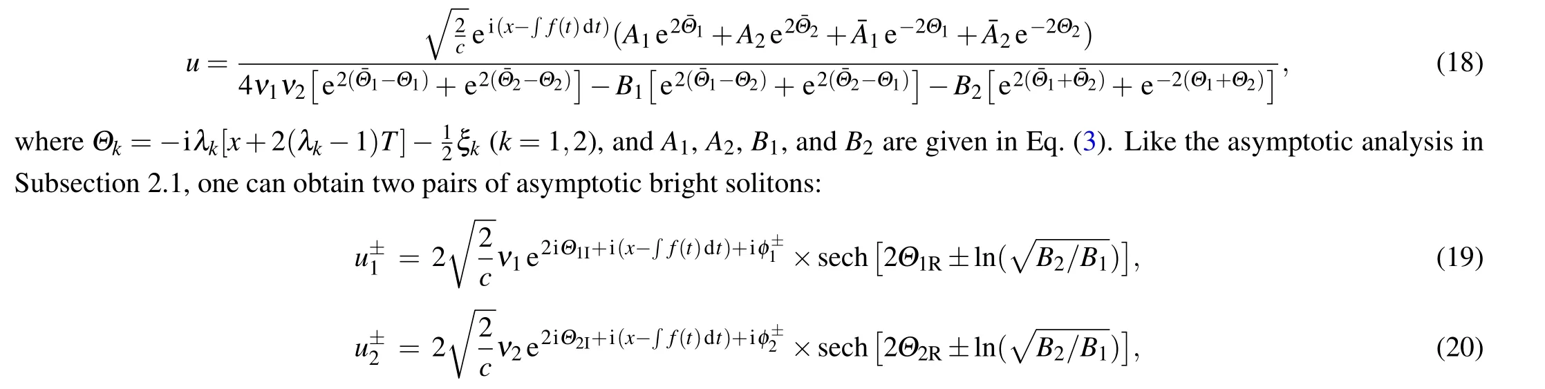
In the cases whenμ1/=μ2, the mutual interaction of two solitons having different velocities is shown in Fig. 1.Via the asymptotic analysis,[8,13]one can derive the expressions of two interacting solitons as|t|→∞by assuming Re(θ1)=O(1) and Re(θ2)=O(1), respectively. Note that when Re(θk)=O(1) there must be|Re(θ3-k)|=∞as|t|→∞fork= 1,2. For convenience, we assume thatν1＞0,ν2＜0, andμ1＞μ2, and use the subscripts “R” and “I” to denote the real and imaginary parts ofθk. From the differenceν2θ1R-ν1θ2R=4ν1ν2(μ1-μ2)t+O(1), one can see that ifθ1R=O(1), thenθ2R→±∞ast →±∞, and that ifθ2R=O(1), thenθ1R→±∞ast →±∞. Thus, two pairs of asymptotic expressions are derived as follows:

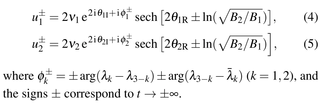
Fig.1. Density plot of solution (3) with λ1 =1+ i, λ2 =-1- i,ξ1=ξ2= ln2+i.

The asymptotic expressions(4)and(5)suggest that solution(3)can describe the elastic two-soliton interaction,that is,the two interacting solitons retain their shapes, velocities and amplitudes upon interaction. But each soliton will experience the phase and position shifts which are respectively as follows:

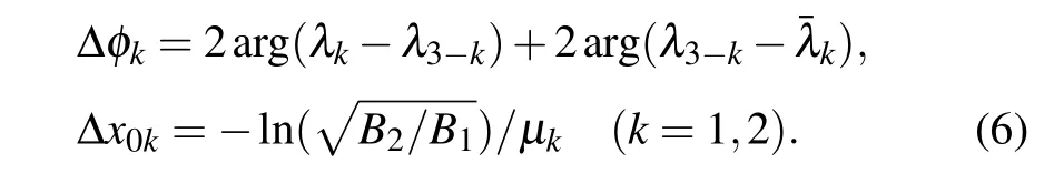
Besides, the soliton center trajectories are along the straight lines 2θkR±ln()=0(k=1,2),so the two interacting solitons diverge from each other linearly as|t|→∞and there is no interaction force.

2.2. Double-pole solution

We should mention that solution (3) cannot describe the interaction of two solitons having the same amplitudes and velocities, which corresponds to that the spectral parametersλ1andλ2merge into the same valueχ. By assumingλ1=χ+ε,λ2=χ-ε, the limit of solution (3) atε →0 can yield the double-pole solution:[40]

whereμ=Re(χ),ν=Im(χ),ξands1are arbitrary constants in C. In such special case, the center trajectories of two solitons are apparently bent but they tend to be parallel as|t|→∞,as shown in Fig. 2. Next, we also use the asymptotic analysis to reveal the dynamical properties of soliton interactions in solution(7),and without loss of generality assumeν ＞0.

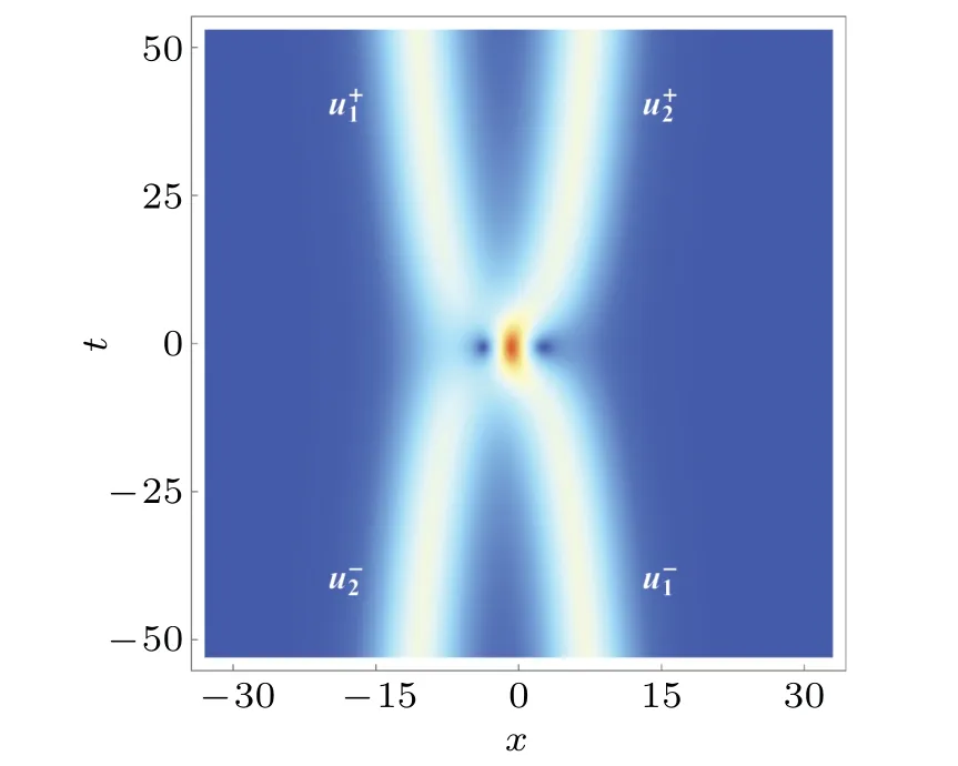
Fig.2. Density plot of solution(7)with χ =i,ξ = ln2+i,s1= i.

Let us useℓto stand for the line directionx-ct=O(1)in thextplane. By making the differenceθR-ν(x-ct)=ν(c+4μ)t+ξR, we know that|θR|→∞withc/=-4μandθR=O(1) withc=-4μalongℓas|t|→∞. However, the asymptotic limits of solution (7) alongℓas|t|→∞always produce 0, which means that solution (7) has no asymptotic soliton lying in any straight line. Thus, we have to discuss the possibility of asymptotic solitons located in certain curves whentand eθR meet some asymptotic balance.

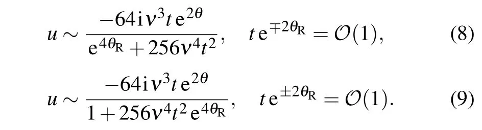
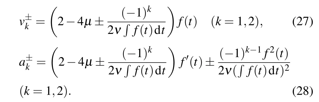
Specifically, we obtain that there are two pairs of asymptotic solitons in solution(7)as follows:

whereu±krepresent the bright asymptotic solitons with their center trajectories located in the logarithmic curves:2θR±(-1)k-1ln（±16ν2t）=0(k=1,2).Since solution(7)is associated to the spectral parameterχ,both two pairs of asymptotic solitons enjoy the same amplitudes=2ν. For each pair of asymptotic solitons (,), the phase and position shifts can be,respectively,characterized by

where the position shift shows the logarithmical growth with|t|. The velocities of asymptotic solitons(k= 1,2) are given by

It can be seen thattend to the common limit-4μat the rateO(t-1) (see Fig. 3(a)), and the values ofv+katt ＞0 are equal tov-katt ＜0(k=1,2). Hence,the soliton interactions in the double-pole solution(7)are still elastic.

By taking the derivatives ofaboutt, we obtain the soliton accelerations=±(1/2νt2) and=∓(1/2νt2).According to Newton’s second law of motion,the two-soliton interaction force can be measured by

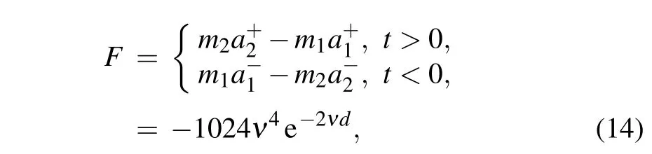
wheremk=dx=4ν(k=1,2)are the soliton masses,andd= ln(16ν2|t|)/νis the relative distance between two solitons. Here,F ＜0 says that the interaction force is attractive and its strength decays exponentially to 0 as the relative distance increases(see Fig.3(b)),which was first obtained in Ref.[37].

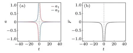
Fig.3. (a)Soliton accelerations versus t;(b)soliton interaction force versus t. The parametric choice follows that in Fig.2.

2.3. Bounded two-soliton solution

Ifμ1=μ2butν1/=ν2, the two solitons can form the bound state because their velocities are associated to the same parameterμ1,2.[10,14]For simplicity, we assume the two solitons have zero velocities by settingμ1,2=0.Then,solution(3)can be reduced to the bounded two-soliton solution:

Depending on the parametersξ1andξ2,solution(15)can display different two-soliton interaction scenarios(see Figs.4(a)–4(c)).In this case,the relationshipν2θ1R-ν1θ2R=O(1)holds in solution(15),which implies thatθ1Randθ2Rhave always the same asymptotic order ast →±∞. As a result,one cannot extract the expressions of interacting solitons in the bound state. Instead,we numerically determine the center positions of the left soliton(u1)and right soliton(u2),and calculate the soliton accelerationsa1anda2. Also,the masses of two solitons can be numerically obtained bymk=dx(k=1,2),where the intervals[ak,bk]are chosen large enough to cover the whole wave packets and require[a1,b1]∩[a2,b2]=∅. Next,we discuss the following three typical cases in solution(15).

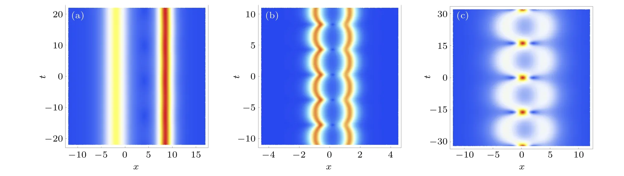
Fig.4. Density plots for three different bounded two-soliton interaction scenarios in solution(15),where the parameters are selected as follows: (a)ξ1=6.9+0.001i,ξ2=ln2+i,ν1= ,ν2= ;(b)ξ1=1+ i,ξ2= ln2+i,ν1=1.9,ν2=2;(c)ξ1=ξ2= ln2+i,ν1= ,ν2=.

(i) If|ξ1|≫|ξ2|, the two solitons are always separated and their relative distance changes very little as the time evolves (see Fig. 4(a)), so that the interaction force is quite weak. For example,whenξ1=6.9+0.001i andξ2=ln2+i, the soliton accelerationsa1,2are within the order 10-2(see Fig. 5(a)) and thus the interaction force is almost 0 (see Fig.5(b)).

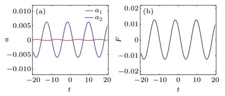
Fig.5. (a)Soliton accelerations and(b)two-soliton interaction force for the case in Fig.4(a).

(ii) If|ξ1|≈|ξ2|, the relative distance between two solitons changes periodically but it will not decrease to 0, which means that they never collide at one point(see Fig.4(b)). For instance, by takingξ1=1+i andξ2=ln2+i, the accelerations of two solitons show the periodical behavior (see Fig. 6(a)). As a result, one can observe the periodic alternating attraction and repulsion between two solitons,which correspond toF ＜0 andF ＞0,respectively(see Fig.6(b)).

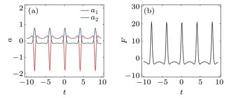
Fig.6. (a)Soliton accelerations and(b)two-soliton interaction force for the case in Fig.4(b).

(iii)If|ξ1|=|ξ2|,the two solitons collide periodically and form a series of transient waves with large amplitudes at interaction points,as shown in Fig.4(c). In this case,the strength of soliton interaction becomes stronger since they collide repeatedly at some moments. Except near the interaction points,we also use the second-order numerical derivatives of relative distance to calculate the soliton accelerations. By takingξ1=ξ2=ln2+i,one can see that the soliton accelerations also exhibit the periodical variation witht(see Fig.7(a)),but the interaction force is of the attractive type in the most of interaction course(see Fig.7(b)).

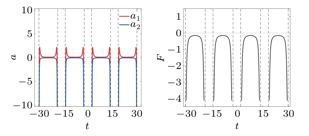
Fig.7. (a)Soliton accelerations and(b)two-soliton interaction force for the case in Fig.4(c).

3. Soliton interactions in the vcNLSE

As we know, equation (2) is integrable under the condition

withcas a real constant, and it can be converted into the standard NLSE iUT+UXX+2|U|2U= 0 via the variable transformations[31]

In this section, we present the exact two-soliton and doublepole solutions of Eq. (2) with condition (16), and quantitatively study the two-soliton interactions with some inhomogeneous dispersion profiles.

3.1. Inhomogeneous regular two-soliton solution

Based on solution (3) and transformation (17), we can obtain the inhomogeneous regular two-soliton solution of Eq.(2):

where(k=1,2) is defined in Eq. (5), and the signs “±”correspond toT →±∞. However,considering that some specificf(t)restricts the sign ofT,one may just obtain one pair of asymptotic solitons asT →∞orT →-∞(see cases(i)and(ii)below).

Interestingly, the soliton velocities and accelerations are dependent onf(t)in the form

and the two-soliton interaction force can be measured by

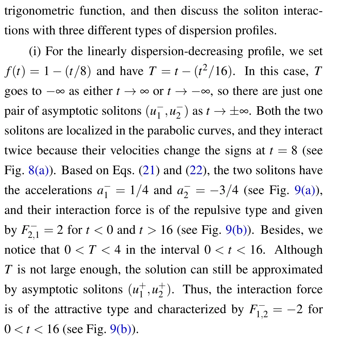
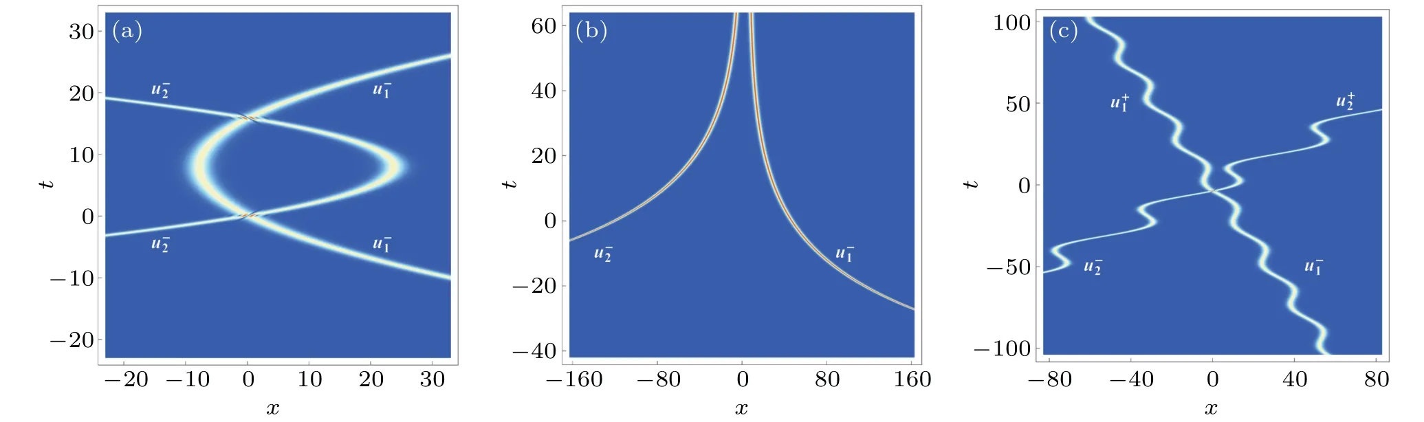
Fig.8.Density plots of inhomogeneous regular two-soliton solution(18)with(a) f(t)=1-t/8,(b) f(t)= e-t/20,(c) f(t)=0.28-0.48sin(0.25t).Other parameters follows those in Fig.1.

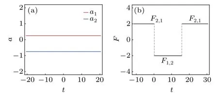
Fig.9. (a)Soliton accelerations and(b)two-soliton interaction force for the case in Fig.8(a).

(ii) For the exponentially dispersion-decreasing profile,we setf(t)= e-(1/20)tand haveT=-20e-(1/20)t. In such a case,Ttends to 0 and-∞respectively ast →±∞, and also there appear just one pair of asymptotic solitons()ast →-∞. The two solitons move along the exponential curves but do not encounter each other becauseTis always smaller than 0 (see Fig. 8(b)). To be specific, the two solitons have the accelerations=(1/10)e-(1/20)tand=-(3/10)e-(1/20)t(see Fig.10(a)).Their interaction force is of the repulsive type and given by=(4/5)e-(1/20)t, which displays the exponential decay whentranges from 0 to-∞(see Fig.10(b)).

Fig.10. (a)Soliton accelerations and(b)two-soliton interaction force for the case in Fig.8(b).

(iii) For the trigonometric dispersion-decreasing profile,we setf(t) = 0.28-0.48sin(0.25t) and haveT= 0.28t+1.92cos(0.25t). In this case,Tgoes to ∞and-∞respectively ast →±∞,so there are two pairs of asymptotic solitons() and () which appear respectively ast →±∞.The asymptotic solitons propagate along the trigonometric periodic curves and experience just one interaction (as shown in Fig. 8(c)). Here, the soliton accelerations can be obtained by= 0.24cos(0.25t) and=-0.72cos(0.25t)(as shown in Fig. 11(a)), and the interaction force is described by expressions=-1.92cos(0.25t) fort ＞0 and=1.92cos(0.25t)fort ＜0,which show the periodical alternation between the attractive and repulsive types(as shown in Fig.11(b)).

Fig.11. (a)Soliton accelerations and(b)two-soliton interaction force for the case in Fig.8(c).

3.2. Inhomogeneous double-pole solution

Similarly, by using solution (7) and transformation (17),we obtain the inhomogeneous double-pole solution of Eq.(2)as follows:

where the signs “±” correspond toT →±∞(Again, one should note that some specificf(t) may cause just one pair of asymptotic solitons appear asT →∞orT →-∞).

where the latter shows the dependence onf(t). Moreover,the soliton velocities and accelerations are respectively obtained by

Thus,the two-soliton interaction can be measured by

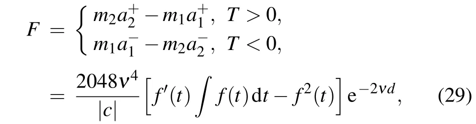
where

are the soliton masses,andd=ln(16ν2(t)dt)/νis the relative distance between two solitons.Also,the force strength exhibits the exponential decay with the relative distance,whereas the force type is related to the sign off′(t)(t)dt-f2(t).

Next, by fixingχ= i/2 and choosingf(t) respectively as a linear function and trigonometric function, we discuss the double-pole soliton interactions with two different types of dispersion profiles.

(i) For the linearly dispersion-decreasing profilef(t)=1-(t/8), the two solitons interact twice at aboutt ≈0 andt ≈16(see Fig.12(a)). BecauseT=t-(t2/16)goes to-∞as botht →∞andt →-∞, the asymptotic solitons ()approach solution(23)well for the intervalst ＜0 andt ＞16.On the other hand,Tis positive in the interval 0＜t ＜16,the asymptotic solitons()can also be used to approximate solution (23) althoughTis not very large. Thus, the soliton accelerations(see Fig.13(a))can be given by

fort ＜0 ort ＞16,

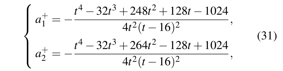
for 0＜t ＜16. Meanwhile, the soliton interaction force is obtained by

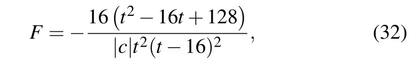
which is of the attractive type in the whole propagation process,as shown in Fig.13(b).

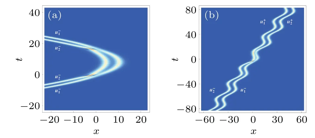
Fig.12. Density plots of solution (18) with (a) f(t)=1-t/8, (b) f(t)=0.28-0.48sin(0.25t). Other parameters are χ = i/2, s1 = 1-(i/2),ξ =(1/2)ln2+(π/4)i and c=1.

Fig.13. (a)Soliton accelerations and(b)two-soliton interaction force for the case in Fig.12(a).

(ii) For the trigonometric dispersion-decreasing profilef(t)=0.28-0.48sin(0.25t),the two solitons move in the periodic trajectories and interact once at aboutt ≈0. In view thatT →±∞corresponds tot →±∞,the two pairs of asymptotic solitons()and()can approach solution(23)respectively ast →∞andt →-∞. Hence,the soliton accelerations(see Fig.14(a))can be given by

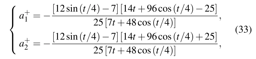
fort ＞0,

fort ＜0,and the soliton interaction force is obtained by

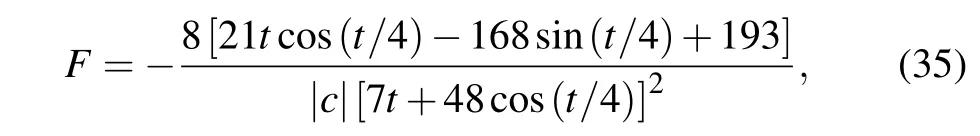
which periodically alternates between the attractive and repulsive types during the propagation process, as illustrated in Fig.14(b).

Fig.14. (a)Soliton accelerations and(b)two-soliton interaction force for the case in Fig.12(b).

4. Conclusions and discussion

In this paper, we have made a quantitative study on the soliton interactions in the NLS equation (1) and its variablecoefficient counterpart(2)based on their exact solutions.

(i) For the regular two-soliton and double-pole solutions (3) and (7) of the NLS equation, we have obtained the expressions of asymptotic solitons ast →±∞via the asymptotic analysis method. Then,we have analyzed the soliton interaction properties by deriving the physical quantities such as amplitudes,phase and position shifts,soliton accelerations,and interaction force. It turns out that the asymptotic solitons in solution(3)exhibit no interaction force,whereas the soliton interaction in solution(7)is attractive and its strength decays exponentially to 0 as the relative distance increases. In addition, for the bounded two-soliton solution, we have numerically calculated the soliton center positions and accelerations,and discussed their interaction scenarios when two solitons are separated with different distances. It shows that the bounded two solitons display the periodic alternating attraction and repulsion,and the interaction strength grows as the relative distance decreases.

(ii)For the vcNLSE(2)with an integrable condition(18),we have obtained the inhomogeneous regular two-soliton and double-pole solutions via the variable transformations (17).Then,we have also derived the expressions of asymptotic solitons, and have quantitatively studied the two-soliton interactions with some inhomogeneous dispersion profiles.Quite differently,we have revealed that the variable dispersion functionf(t)significantly influences the soliton interaction dynamics.On one side,some specificf(t)may cause that only one pair of asymptotic solitons appear asT →∞orT →-∞(see Figs. 8(a), 8(b), 12(a)). On the other side, the functionf(t)plays a major role in determining the soliton interaction types,for example, the regular two-soliton solution may exhibit the repulsive interaction (see Fig. 10(b)), while the double-pole solution may display the periodical alternation between the attractive and repulsive types(see Fig.14(b)).

Acknowledgments

Project supported by the Natural Science Foundation of Beijing Municipality(Grant No.1212007),the National Natural Science Foundation of China (Grant No. 11705284),and the Open Project Program of State Key Laboratory of Petroleum Resources and Prospecting, China University of Petroleum(Grant No.PRP/DX-2211).