Xulong QIN(秦绪龙)

School of Mathematics，Sun Yat-sen University，Guangzhou 510275，China E-mail: qin.xrulong@163.com

Hua QIU(邱华)+

Department of Mathematics，South China Agricultural Universitg，Guangzhou 510642，China E-mail : tsiuhua @scau.edu.cn

Zheng-an YAO (姚正安)

School of Mathematics，Sun Yat-sen University，Guangzhou 510275，China E-mail : mcsyao@mail.sgysu.edu.cn

The magnetic B´enard problem as a toy model derives from the convective motions in a heated and incompressible fluid. As we know, in a homogenous, viscous and electrically conducting fluid,the convection will occur if the temperature gradient passes a certain threshold in two horizontal layers and the convection is permeated by an imposed uniform magnetic field,normal to the layers, and heated from below. The magnetic B´enard problem illuminates the heat convection phenomenon under the presence of the magnetic field (see [8, 9]). It is known for a long time about the global-in-time regularity in two-dimensions of the magnetic B´enard problem under the case ν,µ,κ>0 [2]. The global well-posedness of two-dimensional magnetic B´enard problem with zero thermal conductivity was obtained in[17]. Subsequently,the authors[1] established the global well-posedness of two-dimensional magnetic B´enard problem without thermal diffusivity and with vertical or horizontal magnetic diffusion. Moreover, they proved global regularity and some conditional regularity of strong solutions with mixed partial viscosity.Very recently, the authors [7] proved the local-in-time of strong solutions in the ideal case. For more discussions, we refer to [6, 14, 15] and the references therein.

As b=θ =0,system(1.1)reduces to the standard incompressible Navier-Stokes equations.There are many works about the Navier-Stokes equations. Existence,uniqueness and regularity of solutions about the Navier-Stokes are related to [3, 4, 12] and references therein. It is mentioned that, in 1994, Ponce, Racke, Sideris and Titi [10] proved the global stability of large solutions to the 3D Navier-Stokes equations. Precisely, they proved the global stability of the strong solutions to Navier-Stokes on bounded or unbounded domains under suitable conditions. Later, Zhao-Li [16] and Li-Jiu [5] considered the global stability for large solutions to the evolution system of MHD type describing geophysical flow and Boussinesq equations in 3D bounded or unbounded domains, respectively.

To the best of our knowledge, there is no known results for the global stability of solutions to 3D magnetic B´enard problem (1.1). The purpose of the present paper is to prove some stability results related to problem (1.1). Precisely, we will establish the global stability of strong solutions to 3D magnetic B´enard problem in this paper.

Before we state the main results, let us give some notations. For simplicity, we choose ν = µ = κ = 1 and choose ‖·‖ = ‖·‖L2. Throughout this paper, we will always assume that Ω ⊂R3is a domain with boundary ∂Ω uniformly of class C3. Let P : L2(Ω)H be the Helmholtz projection operator,where H denotes a complete space of{u|u ∈(Ω),∇·u=0}in L2(Ω). Applying the operator P to (1.1), we reformulate problem (1.1) as

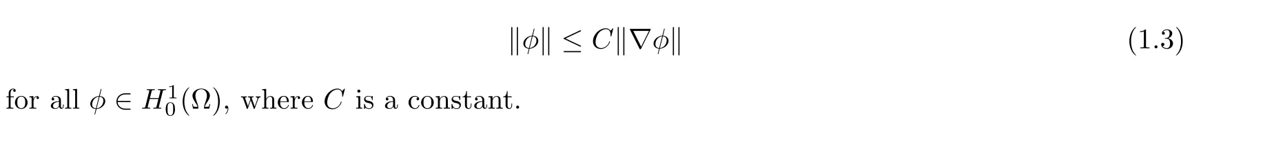
where A = -PΔ is the Stokes operator with domain D(A) = H2(Ω)∩V,V = H10(Ω)∩H,H2(Ω) and H10(Ω) denote the usual Sobolev spaces defined over Ω. For domain Ω bounded or unbounded, we assume that the following Poincar´e inequality holds:

2 The Main Results

In this section, we state our main results as follows:

Theorem 2.1 Let

3 Proofs of Theorems

In this section, we provide the proofs for our main results.

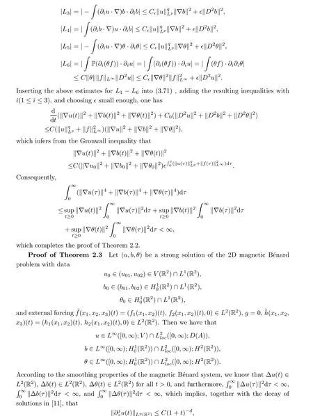
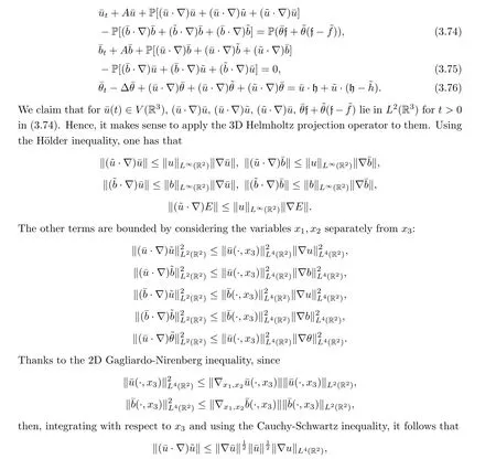
Proof of Theorem 2.1 Under the assumptions made on U0,B0,ϑ0,f,Pg, and h, there exists a local strong solution (U,B,ϑ) of (1.1) for some T = T(‖∇U0‖,‖∇B0‖,‖∇ϑ0‖) > 0,where U ∈L∞((0,T);V)∩L2((0,T);D(A)), B ∈L∞((0,T);V)∩L2((0,T);D(A)), and ϑ ∈L∞((0,T);H10(Ω))∩L2((0,T);H2(Ω)). This observation shows that in order to extend solutions globally, it is sufficient to control‖∇U(t)‖, ‖∇B(t)‖, and ‖∇ϑ(t)‖ uniformly on the interval of local existence. For this purpose, let=U -u,=B-b,=ϑ-θ. Then, (,,) satisfies

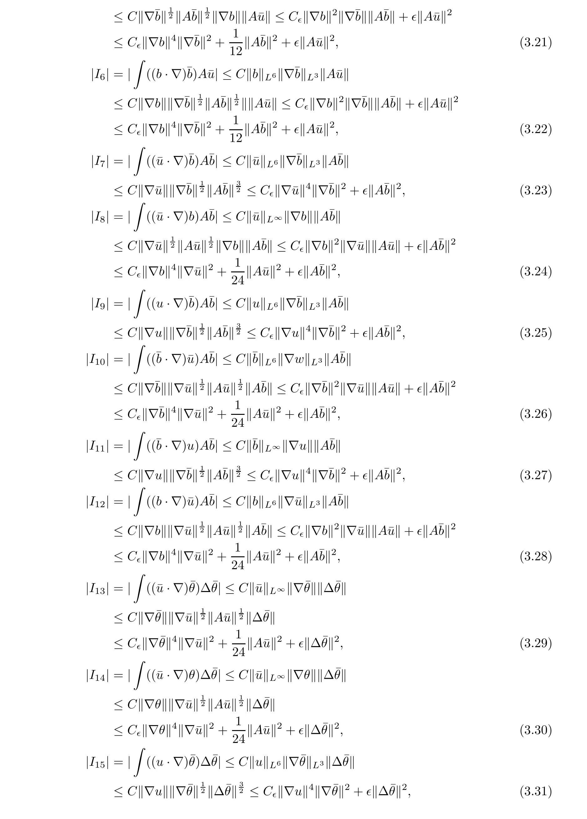
In order to estimate the terms I1-I18, we need to collect a few interpolation inequalities for functions φ ∈D(A). Firstly, under the assumption that ∂Ω is uniformly C3, it was shown in Lemma 1 of [10] that ‖∂2ijφ‖≤C(‖Aφ‖+‖∇φ‖). Since D(A)⊂PL2(Ω), we may integrate by parts and use the Cauchy-Schwarz inequality to get

one can conclude that ‖∇U(t)‖,‖∇B(t)‖ and ‖∇ϑ(t)‖ are uniformly bounded on the domain of definition. Using the continuity method, the solution (U,B,ϑ) to (1.1) exists globally on(0,∞)for t. The remaining statements in Theorem 2.1(i)are now obvious. δ in(2.2)is chosen according to (3.37).

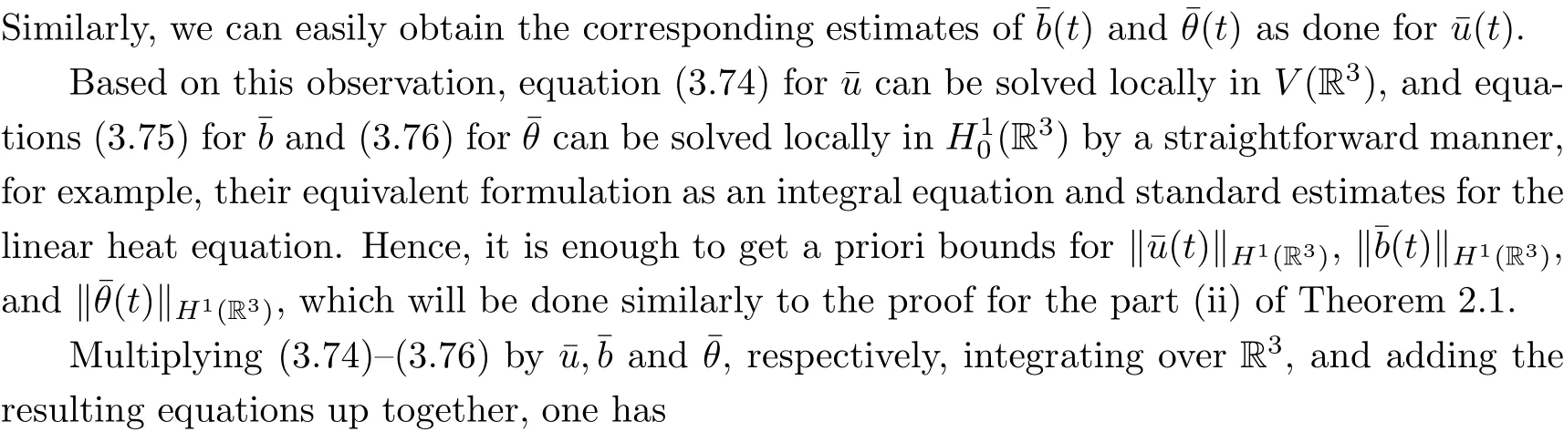
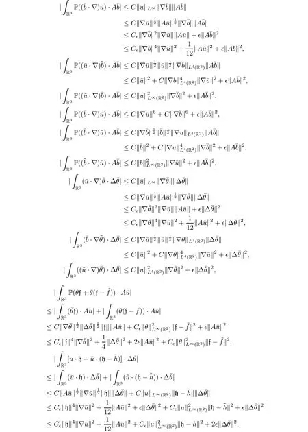
Now we turn to the general case (ii), where the domain Ω satisfy (3.13) and (3.15). Multiplying (3.1)-(3.3) by,and, respectively, and integrating over Ω, we have

Inserting the above estimates for I1-I18into (3.7) and choosing ∊sufficiently small, it gives that

then, combining the above estimates with (3.79) and choosing ∊small enough, it follows that