Guangjun SHEN(申广君)Wentao XU(徐文涛)

Department of Mathematics，Anhui Normal Universitg，Wuhu 241000，China E-mail : gjshen@163.com; wentaoxu1@163.com

Jiang-Lun WU (吴奖伦)*

Department of Mathematics，Computational Foundry Swansea University，Suansea,SA1 8EN，UK E-mail : j.l.wu@swansea.ac.uk

Meanwhile, the averaging principle provides a powerful tool in order to strike a balance between realistically complex models and comparably simpler models which are more amenable to analysis and simulation. The fundamental idea of the stochastic averaging principle is to approximate the original stochastic system by a simpler stochastic system; this was initiated by Khasminskii in the seminal work [7]. To date, the stochastic averaging principle has been developed for many more general types of stochastic differential equations (see, e.g., [4, 10, 11,16, 17, 19, 21], just to mention a few).

Although there are many papers in the literature devoted to study of the stochastic averaging principle for stochastic differential equations with or without delays and driven by Brownian motion,fractional Brownian motion,and L´evy processes,as well as more general stochastic measures inducing semimartingales and so on (see, e.g., [16] and references therein), as we know,there has not been any consideration of an averaging principle for stochastic differential equations driven by time-changed L´evy noise with variable delays. Significantly though,due to their stochasticity,the stochastic differential equations with delays driven by time-changed L´evy processes are potentially useful and important for modelling complex systems in diverse areas of applications. A typical example is stochastic modelling for ecological systems, wherein timechanged L´evy processes as well as delay properties capture certain random but non-Markovian features and phenomena exploited in the real world (see, e.g., [2]). Compared to the classical stochastic differential equations driven by Brownian motion, fractional Brownian motion, and L´evy processes, the stochastic differential equations with delays driven by time-changed L´evy processes are much more complex,therefore,a stochastic averaging principle for such stochastic equations is naturally interesting and would also be very useful. This is what motivates the present paper, which aims to establish a stochastic averaging principle for the stochastic differential equations with delays driven by time-changed L´evy processes. The main difficulty here is that the scaling properties of the time-changed L´evy processes are intrinsically complicated, so it is difficult to construct the approximating averaging equations for the general equations. One remedy for this is to select the involved noises in a proper scaling pattern,and then to establish the averaging principle by deriving the relevant convergence for the averaging principle. In this paper, based on our delicate choice of noises, we succeed in showing that the stochastic differential equations with delays driven by time-changed L´evy processes can be approximated by the associated averaging stochastic differential equations both in mean square convergence and in convergence in probability.

with the initial value x(0) =ξ = {ξ(θ): -τ ≤θ ≤0}∈C([-τ,0];Rn) fulfilling ξ(0) ∈Rnand E‖ξ‖2＜∞, where the functions f :[0,T]×R+×Rn×Rn→Rn, g :[0,T]×R+×Rn×Rn→Rn×m, h : [0,T]×R+×Rn×Rn×(Rn{0}) →Rnare measurable continuous functions,δ :[0,T]→[0,τ], and the constant c>0 is the maximum allowable jump size.

The rest of the paper is organised as follows: in the next section,we will present appropriate conditions to the relevant SDEs(1.1)and briefly formulate a time-changed Gronwall’s inequality in our setting for later use. Section 3 is devoted to our main results and their proofs. In Section 4, the last section, an example is given to illustrate the theoretical results in Section 3.

2 Preliminaries

In order to derive the main results of this paper,we require that the functions f(t1,t2,x,y),g(t1,t2,x,y) and h(t1,t2,x,y,z) satisfy the following assumptions:

Assumption 2.1 For any x1,x2,y1,y2∈Rn, there exists a positive bounded function φ(t) such that

Lemma 2.3 (Time-changed Gronwall’s inequality [20]) Suppose that D(t) is a β-stable subordinator and that Etis the associated inverse stable subordinator. Let T > 0 and x,v :Ω×[0,T]→R+be Ft-measurable functions which are integrable with respect to Et. Assume that u0≥0 is a constant. Then, the inequality

3 Main Results

In this section, we will study the averaging principle for stochastic differential equations driven by time-changed L´evy noise with variable delays. The standard form of equation (1.1)is

Here the measurable functions f, g, h satisfy Assumption 2.2.

Theorem 3.1 Suppose that Assumptions 2.1 and 2.2 hold. Then, for a given arbitrarily small number δ1> 0, there exist L > 0, ∊1∈(0,∊0] and β ∈(0,α-1) such that, for any∊∈(0,∊1],

By Assumption 2.1 and the Burkholder-Davis-Gundy inequality (Jin and Kobayashi [6]), we have

This completes the proof. □

Remark 3.2 We would like to point out that the classical stochastic averaging principle for SDEs driven by Brownian motion deals with the time interval [0,∊-1], while what we have discussed here was a strictly shorter time horizon [0,∊-β] ⊂[0,∊-1] for β ∈(0,α- 1). In other words, the order of convergence here is ∊-β, which is weaker than the classical order of convergence ∊-1. Thus, our averaging principle is a weaker averaging principle. This weaker type averaging principle has been examined for various SDEs by many authors. Essentially,this is due to the fact that the regularity of trajectories of the solutions of SDEs with more general noises is weaker than that of the solutions of SDEs driven by Brownian motion. It is clear that the classical averaging principle for our equation cannot be derived by the method we used here. Of course, to establish a classical averaging principle for our equation is interesting but challenging, so one needs to seek an entirely new approach. We postpone this task to a future work.

4 Example

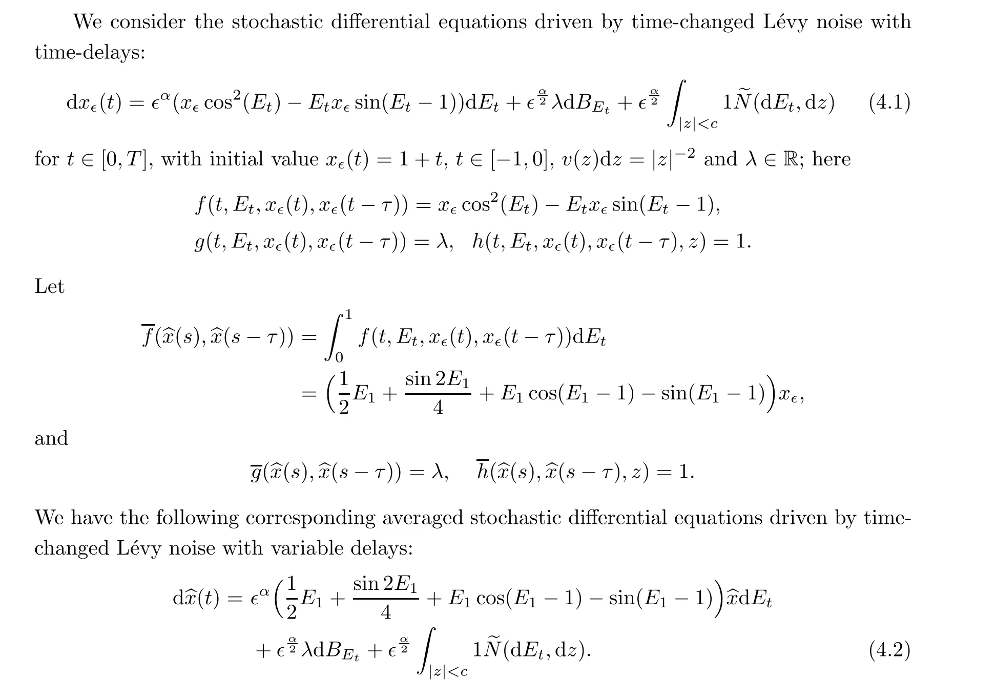
Define the error Err= [|x∊(t)-x∊(t)|2]12. We carry out the numerical simulation to get the solutions (4.1) and (4.2) under the conditions that α = 1.2,∊= 0.001, λ = 1 and α = 1.2,∊= 0.001, and λ = -1 (Figure 1 and Figure 2). One can see a good agreement between the solutions of the original equation and the averaged equation.

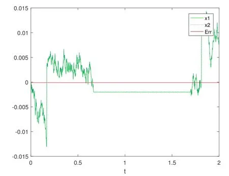
Figure 1 Comparison of the original solution x∊(t) with the averaged solution x(t) with ∊=0.001, λ=1

Figure 2 Comparison of the original solution x∊(t) with the averaged solution x(t) with ∊=0.001, λ=-1