LI Hui WANG Runze WANG Chi

Abstract The local time dependence of the geomagnetic disturbances during magnetic storms indicates the necessity of forecasting the localized magnetic storm indices. For the first time, we construct prediction models for the SuperMAG partial ring current indices (SMR-LT), with the advance time increasing from 1 h to 12 h by Long Short-Term Memory (LSTM) neural network. Generally, the prediction performance decreases with the advance time and is better for the SMR-06 index than for the SMR-00, SMR-12, and SMR-18 index. For the predictions with 12 h ahead, the correlation coefficient is 0.738, 0.608, 0.665, and 0.613, respectively. To avoid the over-represented effect of massive data during geomagnetic quiet periods, only the data during magnetic storms are used to train and test our models, and the improvement in prediction metrics increases with the advance time. For example,for predicting the storm-time SMR-06 index with 12 h ahead, the correlation coefficient and the prediction efficiency increases from 0.674 to 0.691, and from 0.349 to 0.455, respectively. The evaluation of the model performance for forecasting the storm intensity shows that the relative error for intense storms is usually less than the relative error for moderate storms.

Key words Geomagnetic storm, Partial Ring Current Index (PRCI), Artificial Neural Network (ANN)

0 Introduction

Geomagnetic storms are violent global disturbances in the Earth’s magnetosphere, which are one of the consequences of enhanced solar wind-magnetosphere energy coupling through the magnetic reconnection mecha-[1–2]drops rapidly to its minimum value with intense fluctuations (main phase). Finally, along with the decrease of disturbances,Dstrises back to its quiet level slowly (recovery phase).

Geomagnetic storms have been one of the most challenging and passionately explored topics in the geophysical community. This is not only because geomagnetic storms have a significant impact on the global geomagnetic field pattern, but also because they are the most important link in the solar-terrestrial energy coupling chain. Moreover, geomagnetic storms have serious effects on technological infrastructure such as communication systems, electric power systems, oil pipelines, and space vehicles. Therefore, the prediction of geomagnetic storms has important theoretical and practical value.

Researches onDstforecasting have been conducted since the 1970s. Burtonet al.[3]developed an empirical algorithm for forecastingDstusing solar wind velocity and density and the north-south component of the IMF, which contains an approximate description of the effects of solar wind dynamic pressure, particle injection from the plasma sheet, and exponential decay, constrained by ordinary differential equations. Based on this model, several additional assumptions are made to characterize this nonlinear behavior[6–8].

In addition to models constructed based on empirical formulas, there are also researches on forecasting from a data science perspective. One of the widely popular approaches is the construction of machine learning models through Artificial Neural Networks (ANN).Lundstedt and Wintoft[9] developed a feedforward neural network to predict 1 h ahead, using the density and the velocity of the solar wind and the z-component of IMF, which can predict the initial and main phases of magnetic storms. Later an ANN with a specific structure called Recurrent Neural Network (RNN) was introduced to further improve the forecasting effectiveness[10,11]. Different optimization techniques have also been employed for forecasting. Wei et al. [12] used multiscale radial basis networks by changing the activation function of the hidden layer neurons. Lazzús et al. [13]achieved forecasts up to 6 h in advance employing a swarm optimization algorithm. Gruet et al.[14] further achieved better results on forecasting 1～6 h in advance using the Long Short-Term Memory (LSTM) network. Besides, algorithms such ask-Nearest Neighbors(KNN), Nonlinear Auto Regressive Moving Average with eXogenous inputs (NARMAX), and Support Vector Machine (SVM) have been introduced toDstforecasting and other topics in space physics[15–17].

Although theDstindex has a clear physical interpretation, its implicit simplified assumption of azimuthally invariantHperturbations from low or mid-latitude ground stations is not often consistent with observations. A significant dawn-dusk asymmetry ofHdepression tends to occur during storms (see Liet al.[18],and references therein). Given this observed strong Local Time (LT) variations in theH-component at mid-latitude stations, Newell and Gjerloev[19]introduced the SuperMAG Ring current index (SMR index), and Super-MAG partial Ring current indices (SMR-LT indices).SuperMAG is a worldwide collaboration of organizations and national agencies that currently operate more than 300 ground-based magnetometers. Using 98 low and midlatitude magnetometers, the SMR index is conceptually the same as theDstindex, and its local time version, SMR-LT, including SMR-00, SMR-06, SMR-12, and SMR-18, contains local time components named after their respective local time center point, representing midnight, dawn, noon and dusk. The SMR global index is the arithmetic mean of SMR-LT indices.

In this work, we first analyze the asymmetry of SMR-LT indices during geomagnetic storms from several different perspectives. The study of the results shows the importance to predict the SMR region index. We then apply an artificial neural network approach, LSTM,to this topic to provide a forecast of the SMR-LT indices 1～ 12 h in advance. To improve the forecasting performance of the storm-time data, we train a new model using only the data during storms and analyze the model’s performance in predicting the intensity of magnetic storms.

1 Importance of Partial Ring Current Index Prediction

The hourly partial ring current indices, SMR-LT, and the corresponding averaged index, SMR, are obtained from SuperMAG**https://supermag.jhuapl.edu/indices/. During the concerned period from 1998 to 2019, 318 magnetic storms are analyzed.

Liet al.[18]presented a significant dawn–dusk asymmetry ofDstindex during the storm main phase and early recovery phase due to the important contribution of the partial ring current during magnetic storm processes.Fig.1 shows the evolution of partial ring current indices during the magnetic storm on 26 August 2018. As expected, the four SMR-LT indices differ significantly in the main phase and early recovery phase. The depression ofH-components of geomagnetic field disturbances on the dusk side, such as SMR-18 and SMR-12,is generally larger than that on the dawn side, such as SMR-00 and SMR-06. The minimum values of SMR-00,SMR-06, SMR-12, and SMR-18 are –156.9 nT, –155.3 nT, –204.4 nT, and –209.3 nT, respectively. Besides, the SMR-18 index is the earliest to reach its minimum,while the SMR-00 index reaches its minimum one hour later. During the later recovery phase, all the indices are almost the same.

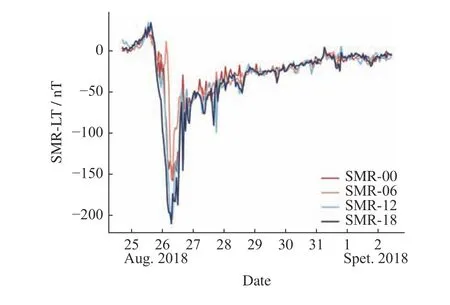
Fig. 1 Partial ring current indices during the magnetic storm on 26 August 2018

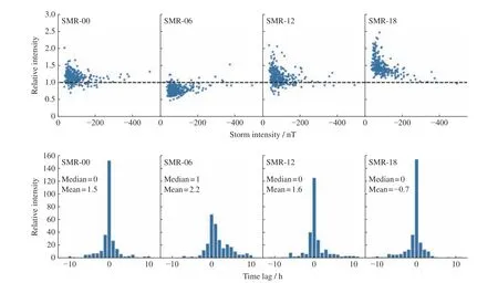
Fig. 2 Statistical characteristics of SMR-LT minimum and its time lag to SMR minimum for 318 magnetic storms

Fig.2 gives the statistical characteristics of SMRLT minimum and its time lag to SMR minimum for 318 magnetic storms. The top panels present the relationship between the relative intensity of SMR-LT indices during storms and the storm intensity, which are defined by the ratio of SMR-LT minimum to SMR minimum and SMR minimum, respectively. Generally, the relative intensity of SMR-18 is greater than 1, indicating a larger geomagnetic depression, while the relative intensity of SMR-06 is less than 1, indicating a smaller geomagnetic depression. The results for SMR-00 and SMR-12 are similar, with the relative intensity greater than 1 in most cases. The mean minimum value of SMR-00, SMR-06,SMR-12, and SMR-18 for the 318 storms is –111.5 nT,–80.7 nT, –109.4 nT, and –133.8 nT, which agrees with the previous results. In addition, the relative intensity for all the four indices tends to be 1 as the storm intensity increases, indicating that the ring current tends to be more symmetric as suggested by Liet al.[18]. Instead of the storm intensity, the onset of storm minimum for the four partial ring current indices also differs from each other. The bottom panels give the distribution of the time lag of SMR-LT minimum to SMR minimum. For SMR-00, SMR-12, and SMR-18, the time lag is concentrated within 1 h. The median values of the time lag are the same, 0. And the mean value is 1.5, 1.6, and –0.7 h,respectively. For SMR-06, the time lag is greater than 0 in many cases, with the median value of 1 h and the mean value of 2.2 h.

Thus, predicting the SMR-LT indices instead of the SMR index is supposed to be more appropriate for regional space weather warning or forecasting.

2 Methodology and Data Set

2.1 LSTM Networks

LSTM is a special kind of RNN. Traditional neural networks cannot deal with time series forecasting. However, RNN can address this issue by designing loops in networks, allowing information to persist and be passed from one step of the network to the next step. An RNN can be regarded as multiple copies of the same network,with messages that can be passed from one copy to a successor copy. The chain-like nature reveals that RNN is intimately related to sequences and lists. However,when the gap between the relevant information and the point where it is needed grows too large, RNN becomes unable to learn to connect the information. The problem is called “long-term dependencies”, explored in depth by Bengioet al.[20], who found it arising from vanishing gradient problems during the training phase of RNN.

LSTM is explicitly designed to avoid the long-term dependency problem. It was introduced by Hochreiter and Schmidhuber[21]and was later refined and popularized by many researchers, making it work tremendously well on a large variety of problems. LSTM also has a chain-like structure, but the repeating module is different. Instead of having a single neural network layer,there are four in LSTM, interacting in a very special approach.

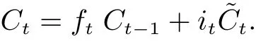
The key to LSTM is the cell state, which runs straight down the entire chain, with only some minor linear interactions. One end of the chain isCt-1, which represents the old cell state, and the other end isCt, which represents the new cell state. The LSTM is designed to remove or add information to the cell state, precisely regulated by structures called gates. Gates are a way to optionally let information through. They are composed of a sigmoid neural net layer and a pointwise multiplication operation. The sigmoid layer outputs numbers between 0 and 1, describing how much of each component should be let through. A value of 0 means completely rejected, while a value of 1 means perfectly accepted.

An LSTM consists of three gates to protect and control the cell state, namely forget gate layer, input gate layer and output gate layer. The forget gate layer is a sigmoid layer to decide what information to be forgotten from the cell state. It receivesht-1andxt, which means the output of the precursor copy and the input of time stept, respectively, and outputs a number between 0 and 1, indicating the extent to which the cell stateCt-1is forgotten. For subsequent equations, the notation is kept thatw*andb*represent the corresponding weights and biases of the layer, respectively.

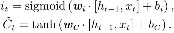
The next step is to decide what new information to be stored in the cell state, which has two parts. First, a sigmoid layer called the “input gate layer” decides which values to be updated. Next, a tanh layer creates a vector of new candidate values,C～t, that could be added to the state.

Finally, the output gate layer will produce a filtered version of cell stateCt. First, a sigmoid layer will be run, which decides what parts of the cell state to output. Then, we put the cell state through tanh (to push the values to be between –1 and 1) and multiply it by the output of the sigmoid gate, so that we only output the parts we decided to.

2.2 Performance Metrics

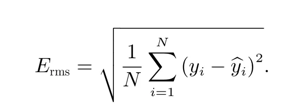
In this study, several performance metrics are used to evaluate the effectiveness of machine learning forecasting models. The root-mean-square error (Erms), is used to represent the error between the observed and predicted values.

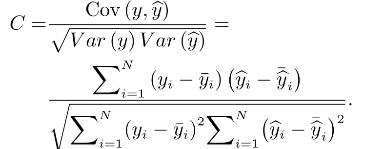
The Pearson correlation coefficient,C, is used to represent the linear relationship between the predictions and the observations. 1/–1 implies a perfect positive/negative correlation, while 0 indicates no linear correlation.

In addition, the prediction efficiency,Pe, is also used and can be calculated as followed.

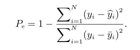
Pe=1 indicates a perfect prediction andPe=0 indicates that the performance of the model is equivalent to the situation by the arithmetic mean of the observation.Pecan be negative values, which in this case means that the model prediction is no better than just taking the arithmetic mean value of the test data. In contrast toC,which only reflects the consistency of the trend of the time series,Pecan also indicate the amplitude of the modeled features, allowing to examine the accuracy of the forecast.

2.3 Data Pre-processing

The solar wind parameters are obtained from OMNI data**https://omniweb.gsfc.nasa.gov**https://supermag.jhuapl.edu/indices/maintained by the National Space Science Data Center (NSSDC) of the National Aeronautics and Space Administration (NASA). The SMR and SMR-LT indices are obtained from SuperMAG collaborators***https://omniweb.gsfc.nasa.gov**https://supermag.jhuapl.edu/indices/.

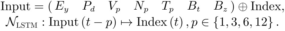
A reasonable selection of feature parameters can make the learning efficiency of ANN greatly improved.In this study, the solar wind fieldEy, the solar wind dynamic pressurePd, the solar wind velocityVp, the solar wind densityNp, the solar wind temperatureTp, the IMF strengthBtand itsz-componentBzare used and denoted byDsw.

The dataset we select from OMNI and SuperMAG spans the period from 1 January 1998, to 31 December 2019, with a temporal resolution of 1 h. The 22 years dataset is divided into three parts, namely the training set(1998－ 2009), the validation set (2010－2014), and the test set (2015－2019). More than a complete solar activity cycle is considered by the training set and the validation set. A total of 257 magnetic storms are identified during these two intervals.

We aim to forecast the SMR-LT indices several hours in advance, denoted asp, which in terms of data structure means developing an LSTM model for multivariate time series forecasting on multiple lag time steps.In this study,p=1,3,6,12 h are considered. The first step is to prepare the dataset for the LSTM, which involves framing the dataset as a supervised learning problem and normalizing the input variables. We frame the supervised learning problem as predicting the SMR-LT index at the current hour given the solar wind parameters on multiple prior time steps. The OMNI data have already been time-shifted from their location of observation to the Earth’s bow shock, which is desired to best support solar wind –magnetosphere coupling studies.Next, we normalize each feature separately to turn the physical quantities into a stream of data that can be processed by the ANN. After the ANN predicts the results,we then apply the scaling process to obtain the true SMR-LT indices.

There are different examples of important design patterns for RNN. We adopt a neural network with recurrent connections between hidden units, that reads an entire sequence and then produces a single output, the SMR index or one of the SMR-LT indices. We construct two hidden layers, the first layer containing 50 neurons and the second layer containing 100 neurons.According to the structural characteristics of the data processed by LSTM, each parameter is a multidimensional vector on the time sequence. The length of the time sequence, denoted bys, can significantly affect the model performance. To evaluate this effect, the results obtained under differentsconditions are given in Fig.3.In general, the model performs best whens=3. Thus,we set the length of the time series to be 3 in the following study, and I nput is, therefore, a 3 ×8 matrix.

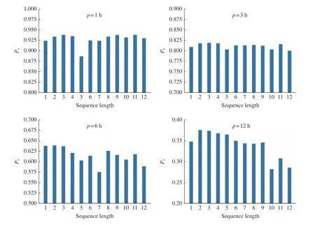
Fig. 3 Performance of models in forecasting the SMR index using different sequence length ( s). The four panels represent the results when different p are considered

3 Results

3.1 Performances of the SMR-LT Indices

Predictions

Given 7 input features of the solar wind, a total of 127 combinations exist. To explore the optimal set of input parameters for eachp, all the possible parameter combinations are tried separately. After comparison, the parameter space,Ey,Pd,Tp,Bt,Bz, performs best and is applied to the prediction.

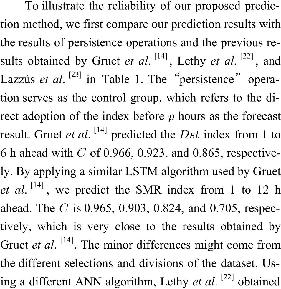
Fig.4 gives the scatter plot of the model’s predictions of SMR-LT indices on the test set. The blue line represents the fitting result, and the black dotted line represents the exact predictions. The closer of the blueline to the black dotted line is, the better prediction results we obtain. It is clear that the predictions are very close to the observations whenp=1. Aspincreases, the deviation of the predictions, mostly undervaluation, to the observations increases accordingly.

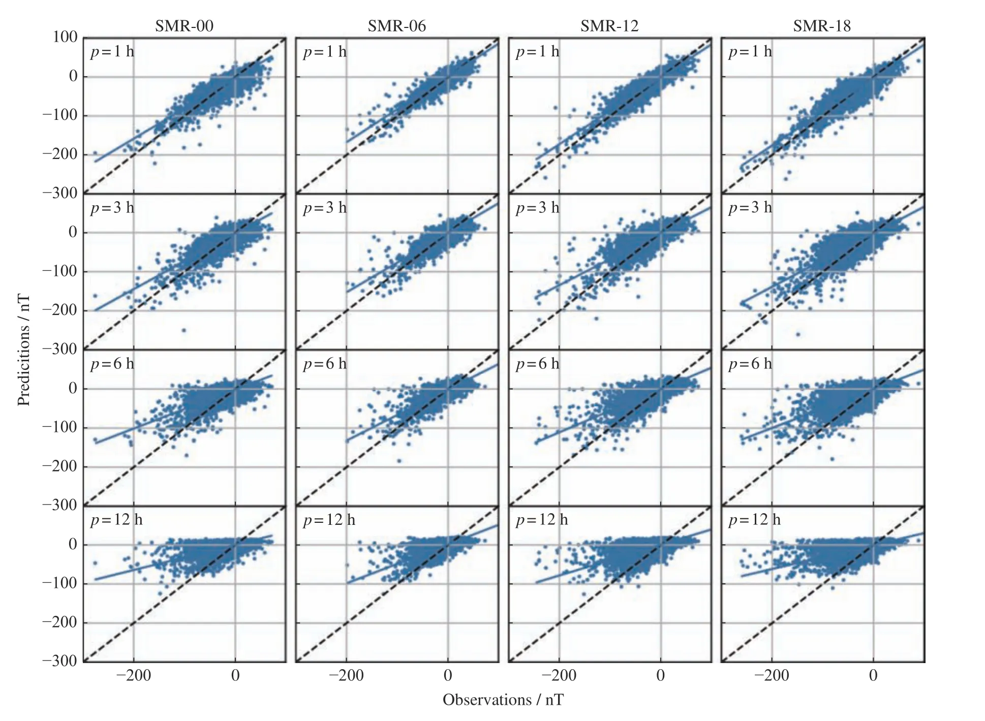
Fig. 4 Scatter plot of the model’s predictions of SMR-LT indices on the test set. The blue line represents the fitting result, and the black dotted line represents the exact prediction

Table 2 gives the quantitative performances of our prediction models for SMR-00, SMR-06, SMR-12, and SMR-18 indices. Considering that there is no previous work on SMR-LT indices predictions, we compare the model predictions with the results of persistence operations to quantitatively represent the model ability. Generally, our model can predict the SMR-LT indices well from the perspectives ofErms,C, andPe. For the prediction of SMR-06 withp=1,3,6,12 h, theErmsis 5.752,6.592, 7.639, and 9.976 nT , respectively, which is 3.4%,17.7%, 22.1%, and 18.0% less than the results of persistence operations; theCis 0.925, 0.873, 0.825, and 0.738,respectively, which is 2.5%, 6.2%, 12.4%, and 25.1%better than the results of persistence operations; thePeis 0.817, 0.759, 0.677, 0.449, respectively, which is 1.6%,17.7%, 44.7%, and 149.4% better than the results of persistence operations. For the prediction of SMR-18 withp=1,3,6,12h, theErmsis 7.316, 10.692, 14.022, and 16.836 nT, respectively, which is 19.3%, 20.9%, 14.0%,and 15.2% less than the results of persistence operations;theCis 0.934, 0.844, 0.743, and 0.613, respectively,which is 4.4%, 10.0%, 12.4%, and 23.1% better than the results of persistence operations; thePeis 0.864, 0.708,0.499, 0.277, respectively, which is 9.4%, 32.6%,55.0%, and 5440.0% better than the results of persistence operations. For the predictions of SMR-00 and SMR-12 index, the results are similar. It is clear that the prediction performances decrease withp, however, the improvements to persistence significantly increase withp.

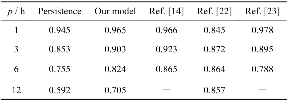
Table 1 Comparison between Ref. [14], Ref. [22],Ref. [23], and our proposed model

3.2 Performances of SMR-LT Index Forecast during Magnetic Storms

The problem of the underestimated predictions shown in Fig.4 might come from the training data structure. In the previous section, all of the dataset is used to train our models. The whole dataset contains a total of 192839 data, of which only 65071 data, or about 33.74%, are during 318 magnetic storms. In the case of intense storms with an intensity of less than –100 nT, there are only 6452 data, accounting for about 3.35%. The overweighting of data during magnetic quiet periods, which is not the focus of the study, might affect the preference of the trained machine learning model, making it always biased to underestimate the intensity of magnetic storms and becomes more prominent for a longer forecast lead time. Thus, although governed by the same fundamental laws of physics, it is still necessary to separate the data during magnetic storms from all-time series from the perspective of data science. Note that, the parameter space with the best performance changes toEy,Pd,Vp,Np,Bt,Bz. Fig.5 shows an example of the predicted SMR-LT indices during the storm on 26 August 2018.Whenp=1,3 h, the predictions are similar to the observations, especially for the SMR-00 and SMR-06 index.Whenp=6,12 h, the deviations of the predictions from the observations are more significant.

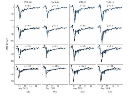
Fig. 5 Evolution of observed (in black) and predicted (in blue) SMR-LT indices during the storm on 26 August 2018

Table 3 gives the quantitative performances of our prediction models for SMR-00, SMR-06, SMR-12, and SMR-18 indices during magnetic storms. “All-time”represents that all the dataset are used to train the model and the metrics are calculated based on the predictions during magnetic storms. However, “storm” represents that only the dataset during magnetic storms is used to train the model and the metrics are calculated based on the predictions during magnetic storms as well. Compared to the results shown in Table 2, theCandPeof both “persistence” and “all-time” have different degrees of reductions due to the removal of the data during magnetic quiet periods, and the reductions increase with the lead time of prediction. At the same time, the results of “storm” are better than the results of “alltime”, and the performance improvement increases with the lead time of prediction. For the prediction of SMR-06 withp=1,3,6,12 h, the improvement ofCis 0.2%,0.3%, 1.4%, and 2.5%, respectively; the improvement ofPeis 3.6%, 1.5%, 4.0%, and 30.4%, respectively. For the prediction of SMR-18 withp=1,3,6,12 h, the improvement ofCis 0.1%, 1.1%, 2.5%, and 8.3%, respectively; the improvement ofPeis –0.1%, –0.6%, 12.2%,and 101.9%, respectively. For SMR-00 and SMR-12 index, the improvements are similar. It is clear that the prediction performances decrease withp, however, the improvements significantly increase withp.

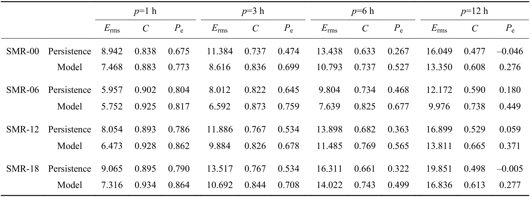
Table 2 Performance of SMR-LT indices forecast

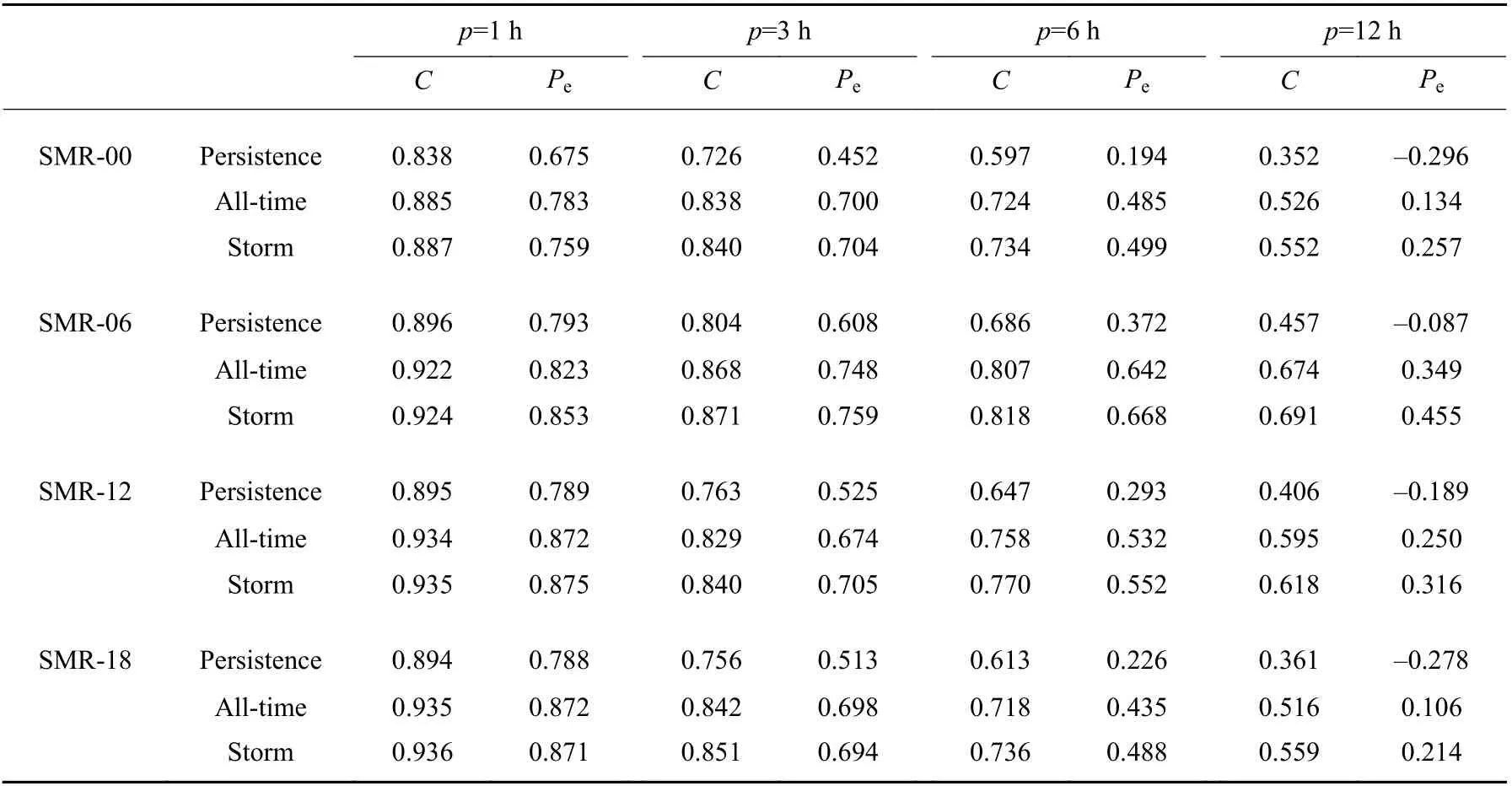
Table 3 Performance of storm-time SMR-LT indices prediction

3.3 Performance of Storm Intensity Prediction

Table 4 gives the distribution of different magnetic storms intensity on the dataset, and Table 5 gives the mean values and standard deviations of the relative errors of storm intensity predictions. There are 61 magnetic storms during the test dataset. All these storms are divided into two groups, moderate storms with the minimum of SMR-LT index between –50 nT and –100 nT,and intense storms with the minimum of SMR-LT index less than –100 nT. Negative values represent underestimations of the storm intensity, while positive values represent overestimations. Note that, the storm intensities in this subsection are discussed in absolute values. It is clear that the relative errors tend to increase with the lead time of predictions. Taking the predictions for SMR-06 index during moderate storms, for example, the relative errors are –10.99%, –13.73%, and –16.88% forp=1,3,6h. During moderate storms, the smallest relative error forp=1 h is for SMR-12 index prediction,–9.81%. Forp=3,6 h, the smallest relative errors are–13.73% and –16.88%, both for SMR-06 index prediction. In contrast, the relative errors for SMR-00 and SMR-18 forecasts are relatively larger, as they tend to have a larger magnitude of variation and are therefore more difficult to predict accurately. In addition, the relative errors for intense storms are relatively less than those for moderate storms.

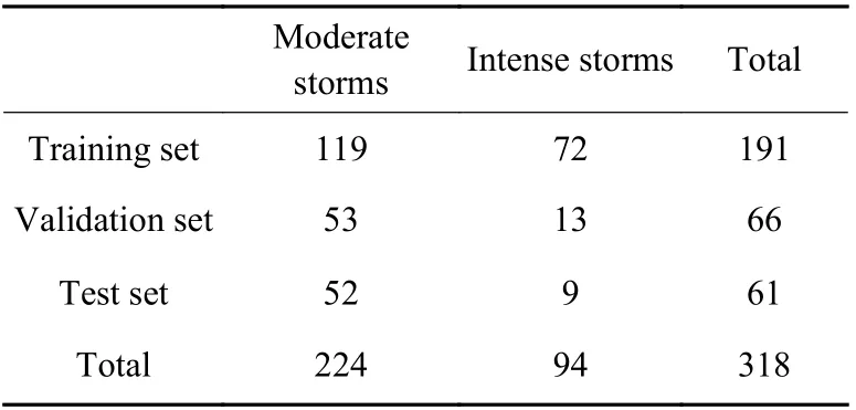
Table 4 Magnetic storm intensity distribution

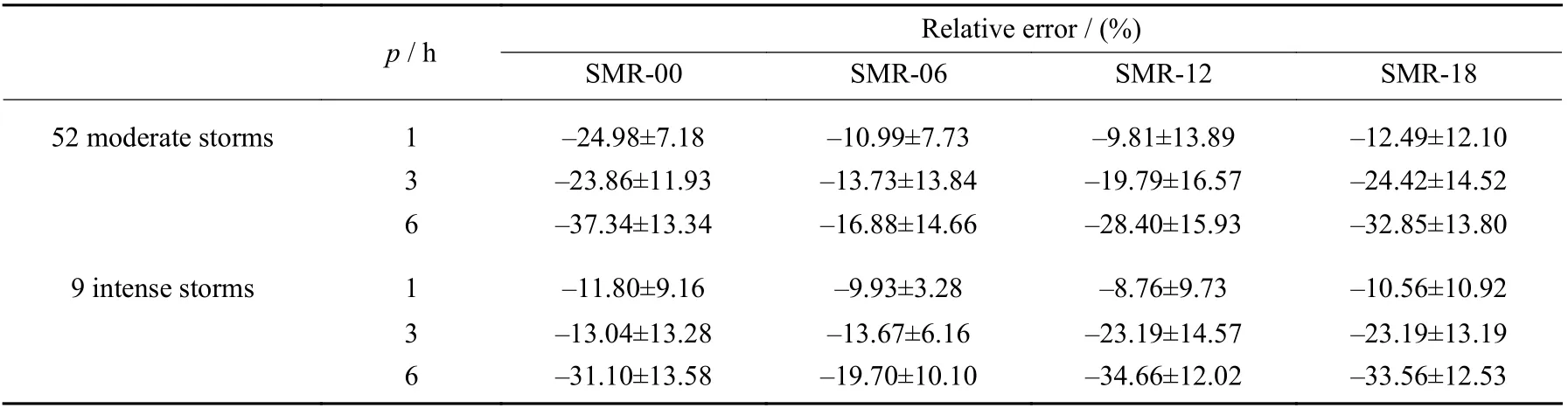
Table 5 Relative errors (mean±standard deviation) of storm intensity predictions

4 Summary

In this paper, we construct models for predicting partial ring current index, SMR-LT, with an advance time from 1 h to 12 hviaLSTM neural networks. Although theDstindex is widely used to present the averaged magnetic disturbances on a global scale, the local time dependence of geomagnetic disturbances during magnetic storms indicates the importance of forecasting localized magnetic storm indices, especially for studying the effects of magnetic storms on a particular region.

Using LSTM neural network, we construct prediction models of partial ring current index, SMR-LT, with an advance time from 1 h to 12 h for the first time. From 127 combinations of 7 solar wind parameters, the parameter space,Ey,Pd,Tp,Bt,Bz, performs best. The performances of the SMR index prediction are comparable with the results of the published models, which validates the reliability of our model when applying it to predict the SMR-LT indices. Generally, the prediction performance decreases with the advance time and is better for SMR-06 than for SMR-00, SMR-12, and SMR-18. For the prediction of SMR-00, SMR-06, SMR-12,and SMR-18 with 12 h ahead, the correlation coefficient is 0.608, 0.738, 0.665, and 0.613, respectively.

The evaluation of the model results shows that the over-represented (over 66.26%) data during magnetic quiet periods might affect the learning preference of the ANN. To avoid the over-represented effect, we filter out the data during magnetic quiet periods from the dataset and train a new model, labeled as the “storm” model.The performance improvement increases with the advance time. Taking the prediction of storm-time SMR-06 index with a 12 h advance time, for example, the correlation coefficient and the prediction efficiency increa-ses from 0.674 to 0.691, and from 0.349 to 0.455, respectively.

We also evaluate the model performance for forecasting storm intensity. The relative errors tend to increase with the lead time of predictions. The relative error of storm intensity prediction for intense storms is usually less than that for moderate storms.

AcknowledgementThe authors thank the SuperMAG collaborators for the use of SMR and SMR-LT indices, which are accessible in https://supermag.jhuapl.edu/indices/ . The OMNI data were obtained from the GSFC/SPDF OMNIWeb interface at https://omniweb.gsfc.nasa.gov. Special thanks to Dr. Tang B B, Dr. Li W Y, and Prof. Guo X C for helpful discussions.