LARGE TIME BEHAVIOR OF THE 1D ISENTROPIC NAVIER-STOKES-POISSON SYSTEM*
2022-11-04
Department of Mathematics,Capital Normal University,Beijing 100048,China
E-mail: qyhe.cnu.math@qq.com
Jiawei SUN (孙家伟)†
Department of Mathematics,Shandong Normal University,Jinan 250014,China
E-mail: sunjiawei0122@163.com
Abstract The initial value problem (IVP) for the one-dimensional isentropic compressible Navier-Stokes-Poisson (CNSP) system is considered in this paper.For the variables,the electric field and the velocity,under the Lagrange coordinate,we establish the global existence and uniqueness of the classical solutions to this IVP problem.Then we prove by the method of complex analysis,that the solutions to this system converge to those of the corresponding linearized system in the L2 norm as time tends to infinity.In addition,we show,using Green’s function,that the solutions to this system are close to a diffusion profile,pointwisely,as time goes to infinity.
Key words 1D Navier-Stokes-Poisson system;well-posedness;L2-time decay rates;timespace pointwise behaviors
1 Introduction
The unipolar isentropic compressible Navier-Stokes-Poisson (CNSP) system can be used to simulate,for instance in semiconductor devices,the transport of charged particles under the influence of the electric field of electrostatic potential force [26].The unipolar isentropic CNSP system is given by
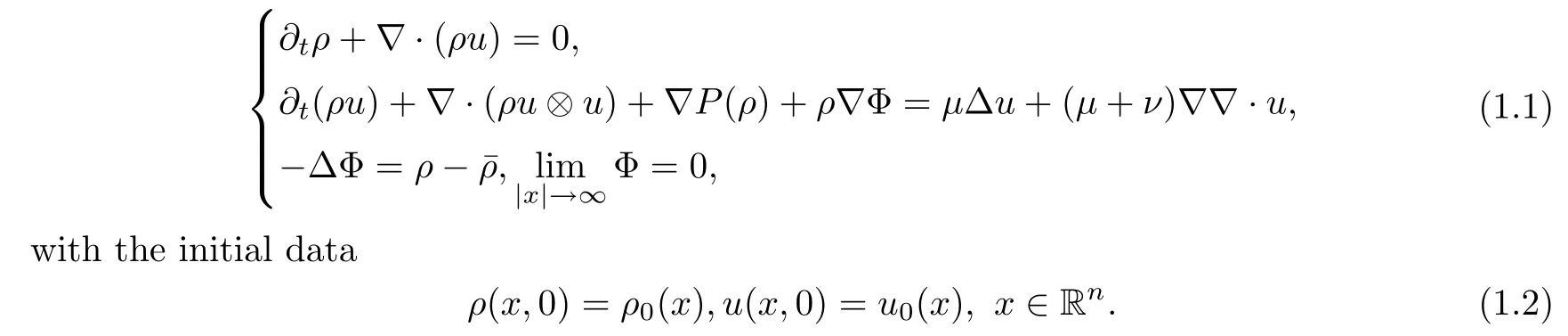
The variables are the densityρ >0,the velocityu,the momentρuand the electrostatic potential Φ.Furthermore,P(ρ)=ργ(γ >1) is the pressure function.The viscosity coefficients satisfyμ >0,2μ+nν >0,the space dimension isn.¯ρ >0 denotes the background doping profile,and,for simplicity,in this paper,is taken as 1.
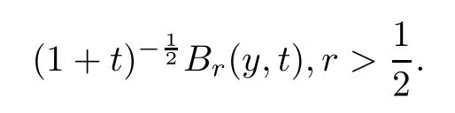
The purpose of this paper is to study the large time asymptotic behaviors of the solutions to the initial value problem (IVP) for the one-dimensional CNSP system,in which both the low dimension and the presence of an electric field give rise to low time decay rates of the solutions to this system.We recall some known results on the time decay rates of the solutions to the IVP for the CNSP system when the initial data (ρ0,u0) is a small perturbation of the constant state (¯ρ,0).Li,Matsumura and Zhang [11] obtained the global existence and the large time behaviors of the classical solutions of the three-dimensional CNSP system by a spectrum method and energy estimates.They mainly found that the density converges to its equilibrium state at the sameL2-time decay rateas the Navier-Stokes system,but that the momentum decays at theL2-time rate.Then they extended similar results to the non-isentropic case [40].On the other hand,in [29,33],Wang and Wu investigated the pointwise estimates of the solutions to the IVP for the CNSP system in multi-dimensions (n≥3),and showed that the pointwise profiles of the solutions contain the diffusion wave with the formfor the density and the formfor the momentum and the electric field,but do not contain the generalized Huygens’ wave with the formthis is different from the cases for the Navier-Stokes system in [15,16].Here,we define

In fact,the CNSP system is a hyperbolic-parabolic system with a non-local term arising from the electric field ∇Φ.It is this non-local term that destroys the time decay rates and the regularities (integrability) on the space variable for the momentum (or the velocity).Recently,under the additional assumption thatand the neutral condition,Wang [32] obtained that theL2-time decay rate of the density is,and for both the velocity and the electric field is (1 +t)-σp,with(1<p≤2),for the three-dimensional CNSP system.Li and Zhang [13]considered a similar problem in the negative Besov space to improve theL2-time decay rates with the neutral condition on initial density.In addition,Wu and Wang [35] improved the timespace pointwise estimates of the solutions for the CNSP system in R3under the same neutral condition.There are many other related results on large time behaviors of solutions perturbing around constant equilibrium for the bipolar CNSP system in multi-dimensions (n≥3);see[12,30,36,37,39].
In this paper,we consider the IVP for the one-dimensional CNSP system with the neutral condition.For the variables,the electric field and the velocity,under the Lagrange coordinate,we first establish the global existence and uniqueness of the classical solutions to the system.Then we consider theL2-time decay estimates and the time-space pointwise estimates of the classical solutions to the system.By the method of complex analysis,as in [11],we prove that theL2-time decay rate of both the electric field and the velocity is,and of the density is.We note that theL2-time decay rates of the solutions to the IVP (1.1)–(1.2) for the one-dimensional CNSP system are the same as the case in R3[11],this is because the neutral condition weakens the effect of the electric field.By using Green’s function as in [16,31],as time goes to infinity,we also prove that the solutions to this system are close to a diffusion profile,pointwisely,with the form
We also look back previous works on the IVP for some related topics and models.For the compressible Navier-Stokes system,a lot of work has been done on the existence,the stability and theLp-time decay rates withp≥2 for either isentropic or non-isentropic (heat-conductive)cases (cf.[1,2,5–10,14,17,24,25,27]) in various settings by using the (weighted) energy method together with spectrum analysis.On the other hand,Liu and Zeng [23] first studied the pointwise estimates of solutions to general hyperbolic-parabolic systems in one space dimension by using the Green’s function method.Hoffand Zumbrun [3] investigated theLp(Rn)(p≥1)estimates for the isentropic Navier-Stokes system in multidimensions.Then,in [4],they deduced a detailed,pointwise description of the Green’s function for the related linearized Navier-Stokes system with artificial viscosity.Later,Liu and Wang [16] considered the pointwise estimates of the solution in odd dimensions,and showed the generalized Huygens’ principle by using a real analysis method;this was reconsidered in [15] by using the complex analysis method for the Green’s function.In particular,Liu and Wang showed in [15,16] that the solution behaves as the superposition of a diffusion wave and a generalized Huygens’ wave.Wang et al.[31,34] also discussed the pointwise estimates of the solution for the dampened Euler system when initial data is a small perturbation of the constant state,and showed that the solution behaves as the diffusion wave since the long wave of the Green’s function does not contain the wave operator.There are also other results using Green’s function in [18–22,28,38,41] on the related models for theL1-time decay estimates,the stability of the boundary layer,and the wave propagation pattern around the shock wave.
NotationsThroughout the rest of this paper,C >0 denotes the generic positive constant independent of time.
2 Model Description and Main Results
We introduce the one-dimensional isentropic CNSP system
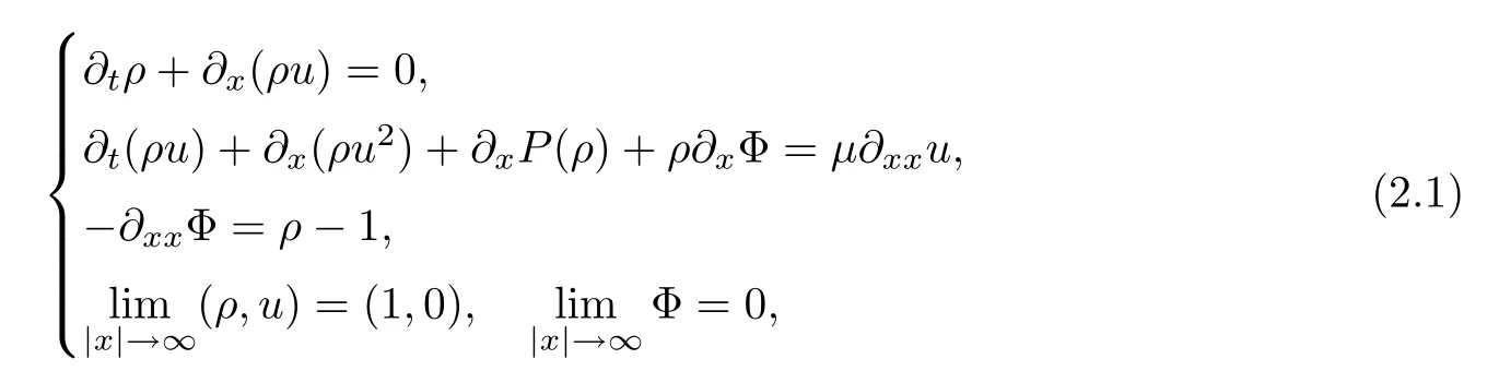
with the initial data

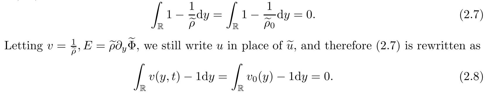
In particular,the density is required in order to satisfy the neutral condition

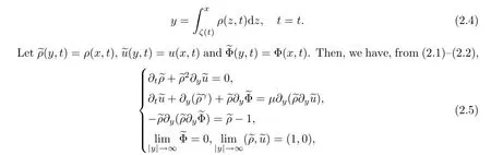
Inspired by [23,41],we will describe the system (2.1)–(2.3) under the Lagrange coordinate.First of all,we introduce a particle path with the velocityufrom the original point
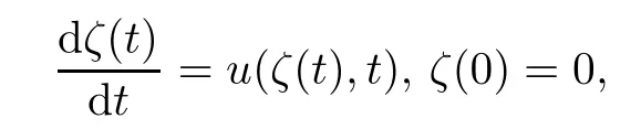
and thus the Lagrange coordinate transform can be defined as
with the initial data

From (2.3),we have that
From the electric field equation (2.5)3,we have that

and combining this with the mass equation (2.5))1,it holds that

which implies that∂tE-u=0.
In conclusion,the one-dimensional CNSP system under the Lagrange coordinate with the neutral condition is expressed as

In this paper,we mainly study the large time asymptotic behaviors of the global classical solutions to the IVP for the system (2.11)–(2.14).We now state the main results of this paper.
To begin with,we establish the global existence and uniqueness of the classical solutions to the IVP (2.11)–(2.14) in the following theorem:
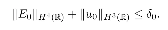
Theorem 2.1(Global existence) Assuming thatE0∈H4(R) andu0∈H3(R),there exists a constantδ0>0 small enough such that
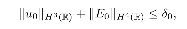
so the IVP (2.11)–(2.14) admits a unique and global solution (E,u) satisfying

for anyT >0.In addition,for anyT >0,we have the following inequality:

We show that the solutions to the system (2.11)–(2.14) converge to those of the corresponding linearized system as time tends to infinity in the following theorem:
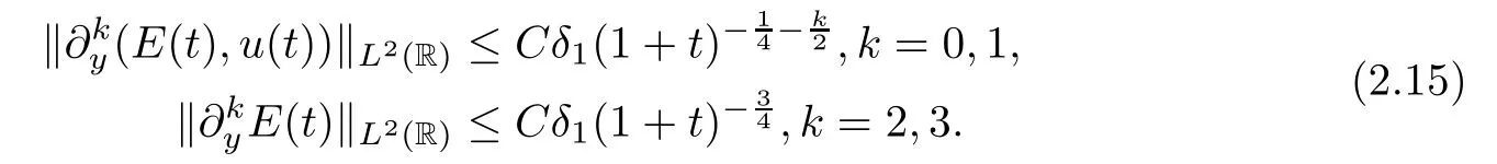
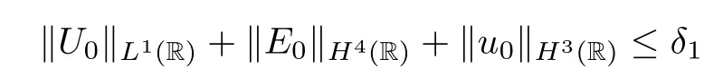
Theorem 2.2(L2-time decay) Assuming thatE0∈H4(R) ∩L1(R) andu0∈H3(R) ∩L1(R),there exists a sufficiently small constantδ1>0 such that

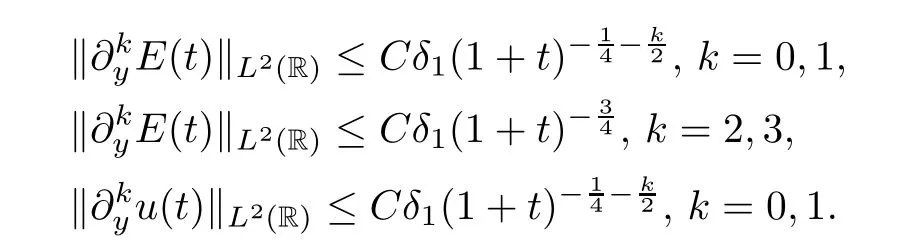
so the global classical solution (E,u) of the IVP (2.11)–(2.14) obtained by Theorem 2.1 satisfies
Assume further that

for some constantsc0>0 and∈0>0.Then,for anyt≥t0witht0>0 being a sufficiently large time,we have that
Remark 2.3We give the example (E0(y),u0(y),ρ0(x)),which satisfies (2.16) and the neutral condition (2.11).Forδ >0 small enough,we set that

From (2.14),we have that

We define a coordinate transformyx:=f(y),y∈R by an ordinary differential equation

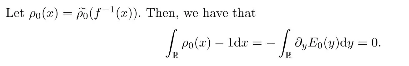
Simply put,ρ0(x) satisfies the neutral condition (2.11) and (E0(y),u0(y)) satisfies (2.16).
In addition,we show in the following theorem that the solutions to the system (2.11)–(2.14)are close to a diffusion profile,pointwisely,as time goes to infinity.
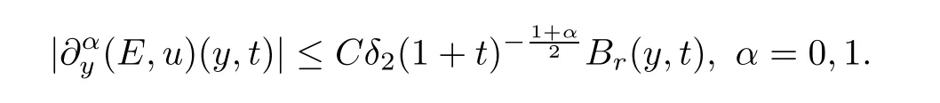
Theorem 2.4(Time-space pointwise behaviors) Assume that the initial data (E0,u0)satisfies the assumptions of Theorem 2.1.Moreover,if,forα=0,1,there exists a sufficiently small constantδ2>0 such that
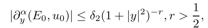
then the global classical solution (E,u) of the IVP (2.11)–(2.14),given by Theorem 2.1,satisfies that
3 Global Existence
In this section,we show the global existence and uniqueness of the classical solutions to IVP (2.11)–(2.14).We first give the global a priori estimates.
Proposition 3.1Assume that there exists a constantδ0>0 small enough such that
Then the global classical solution (E,u) of the IVP (2.11)–(2.14) satisfies that

for anyT >0.
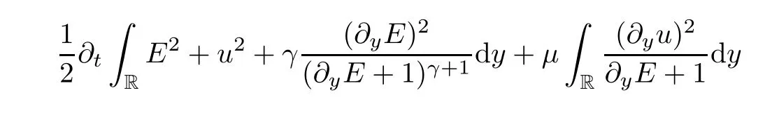
ProofFirst,we try to get the first order regularity,multiplying (2.11) and (2.12) byEandu,respectively,and integrating on R.We obtain that

We estimate the second formula of (3.2) and attain that

We insert (3.3) into (3.2) and obtain that

Multiplying (2.11) and (2.12) by,respectively,and integrating on R,then by integrating by parts,we attain that
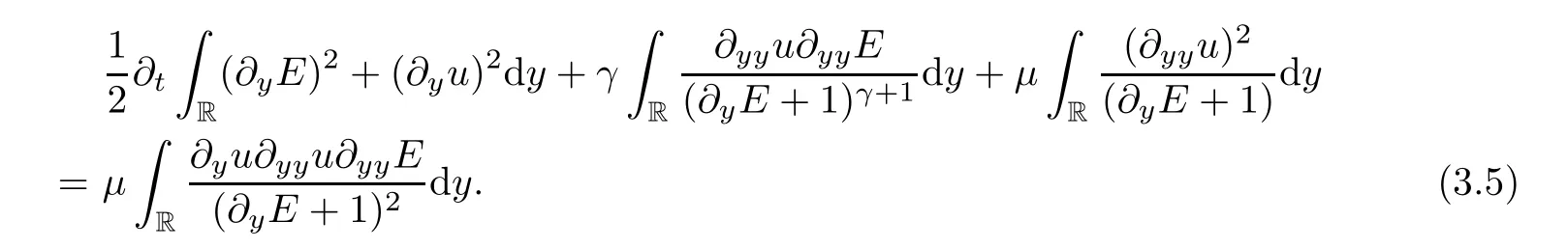
Similarly to (3.3),we estimate the second formula of (3.4) and get that
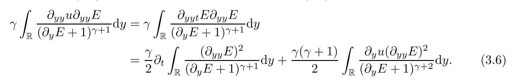
Combining (3.5) and (3.6),it holds that

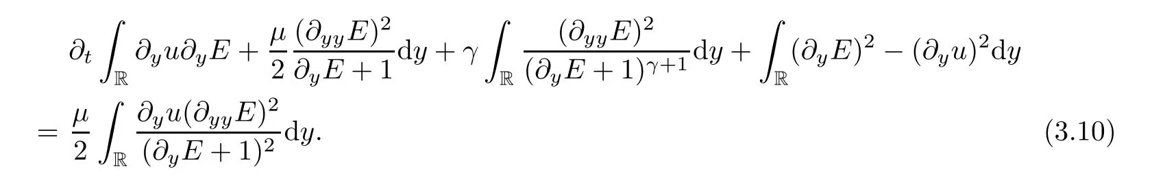
Multiplying (2.11) and (2.12) byE,respectively,and integrating on R,then by integrating by parts,we have that
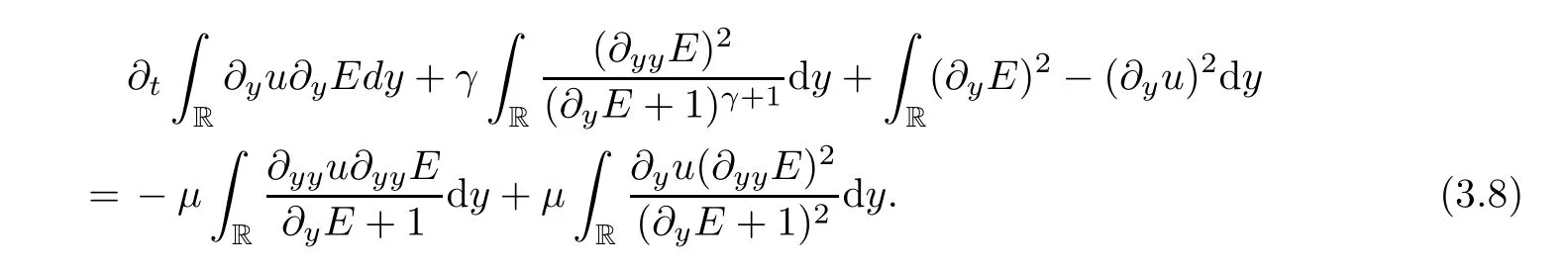
Similarly to (3.6),we obtain that

Taking (3.9) into (3.8),we can get the second order dissipation ofE:
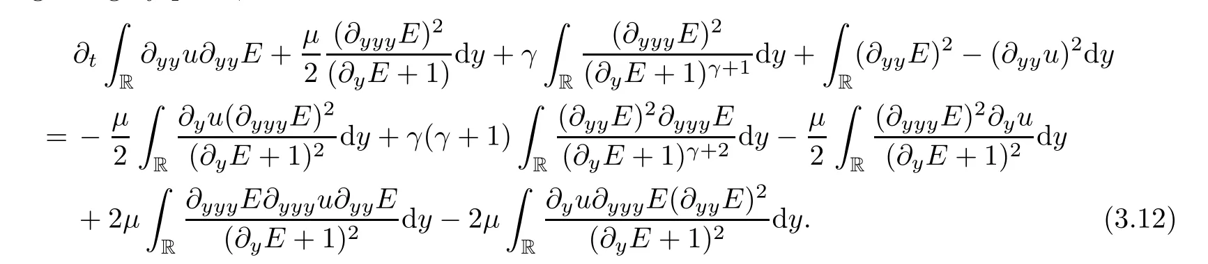
Next,we aim to get high order derivative estimates and omit some similar but more tedious calculation processes,as before.Multiplying (2.11) and (2.12) by,respectively,and integrating on R,then by integrating by parts,we get that
Multiplying (2.11) and (2.12) by,respectively,and integrating on R,then by integrating by parts,we attain that
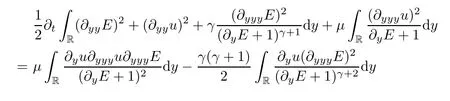
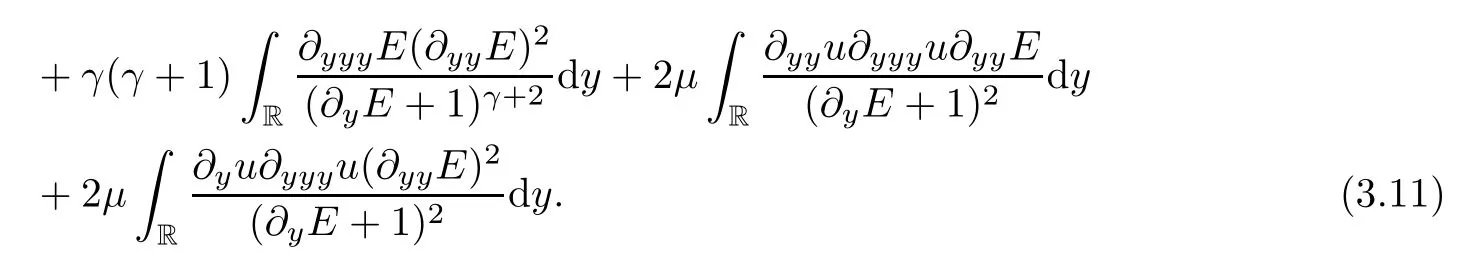
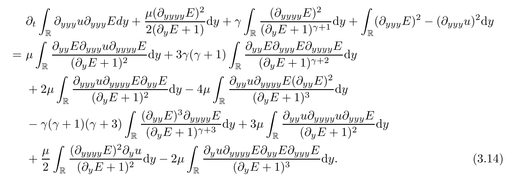
Multiplying (2.11) and (2.12) by,respectively,and integrating on R,then by integrating by parts,we have that
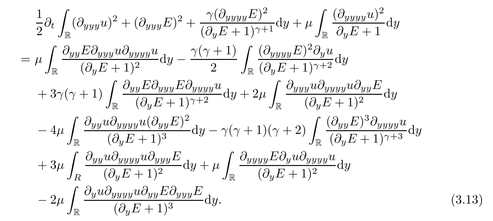
Multiplying (2.11) and (2.12) by,respectively,and integrating on R,then by integrating by parts,we obtain the fourth order dissipation ofE:
Now,two time dependent functions,A(t) and B(t),are given as
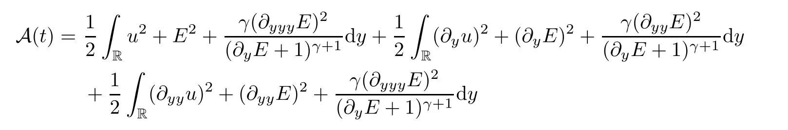
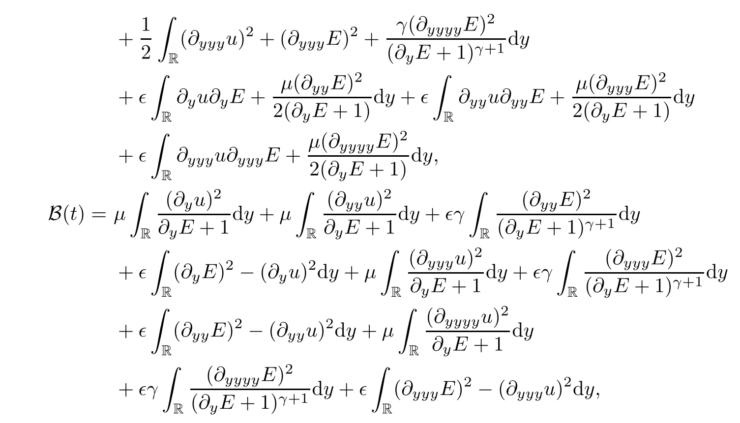
where∈is a small constant.
Forf∈H1(R),we have the following embedding inequality:

Thanks to an a priori smallness assumption,the fact that

and the embedding inequality (3.15),we have that


Using the a-priori smallness assumption,and integrating time on [0,t] for any givent >0,the proof is completed. □
Proof of Theorem 2.1The proof of the local well-posedness of the IVP (2.11)–(2.14) is standard as in [24],so we omit it.With the help of the global a priori estimates in Proposition 3.1,the unique global classical solutions of IVP (2.11)–(2.14) can be obtained by continuity arguments.The proof of Theorem 2.1 is complete. □
4 L2-time Decay Rates
In this section,we aim to prove that the solutions to the IVP (2.11)–(2.14) converge to those of the corresponding linearized system in theL2norm as the time tends to infinity.First,we apply spectral analysis to the semigroup for the linearized CNSP system in Subsection 4.1,then we get theL2-time decay rates of the solutions to this linearized system in Subsection 4.2.We prove that theL2-time decay rates of the solutions to this linearized system are optimal in subsection 4.3.Next,in Subsection 4.4,using the Duhamel’s principle,we reformulate the IVP(2.11)–(2.14).Finally,in Subsection 4.5,we prove that the solutions to the IVP (2.11)–(2.14)converge to those of the corresponding linearized system as the time tends to infinity in theL2norm.
4.1 Spectral analysis of the semigroup
Let us consider the IVP for the linearized isentropic CNSP system
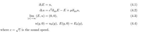
We rewrite (4.1)–(4.4) as

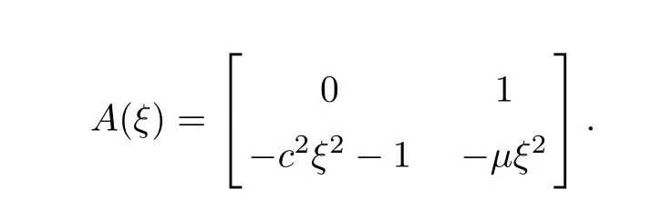
whereA(∂y) is a differential operator matrix

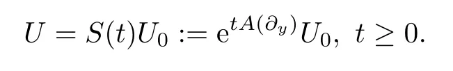
U=(E,u)⊤andU0=(E0,u0)⊤.The solutionUof (4.5) can be expressed as
Applying the Fourier transform to system (4.5),we have that
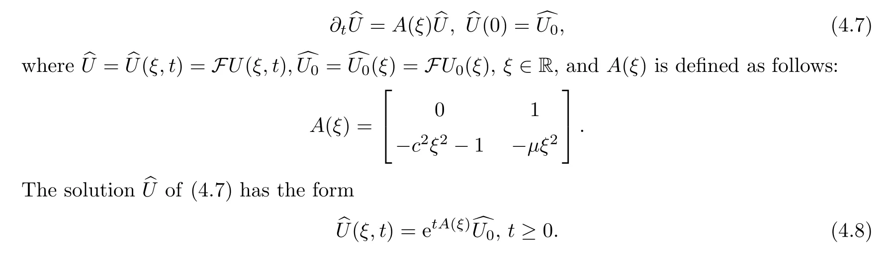
The eigenvalues of the matrixA(ξ) are computed from the determinant

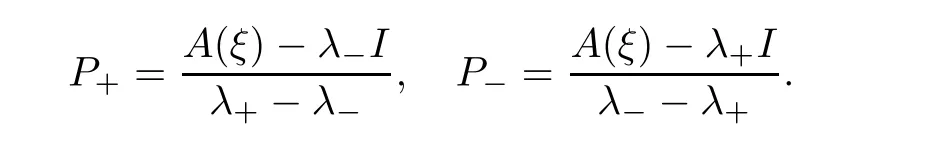
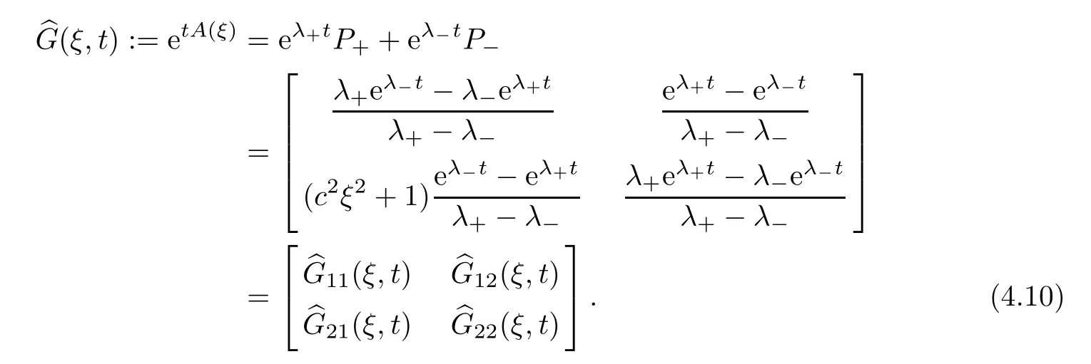
The etA(ξ)is expressed as etA(ξ)=eλ+tP++eλ-tP-,where the projection matricesP+andP-are defined as follows:
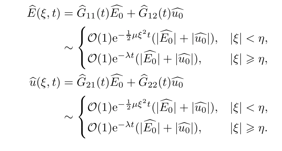
By a direct computation,we can verify that the exact expression of the Fourier transform(ξ,t) of the Green’s functionG(y,t)=etA(∂y)is
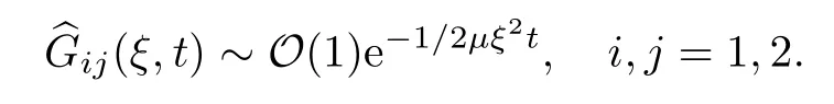
There exists a constantη >0 such that,if |ξ|<η,we obtain that
If |ξ| ≥η,for some given constantλ >0,we have that

4.2 L2-time decay rates for the semigroup
With the help of formula (4.10) and the asymptotic analysis of its elements,we get theL2-time decay rates of the global classical solutions to the IVP for the linearized CNSP system(4.1)–(4.4) as follows:
Proposition 4.1LetE0∈H4(R) ∩L1(R) andu0∈H3(R) ∩L1(R).Then the solutionU=(E,u)⊤of the IVP (4.1)–(4.4) satisfies that

for 0 ≤k≤3.
ProofDue to Parseval’s equality,we have that
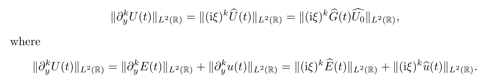
Combining (4.8) and (4.10),an easy computation gives that
Therefore,we can obtain theL2-time decay rates for (E,u) as

wherek=0,1,2,3. □
Remark 4.2From (4.8) and (4.10),since,we can obtain that

4.3 Optimal L2-time decay rates for the semigroup
It should be noted that theL2-time decay rates derived in Proposition 4.1 are optimal.
Lemma 4.3Aside from the assumptions on initial data (E0,u0) as in Proposition 4.1,we also assume that
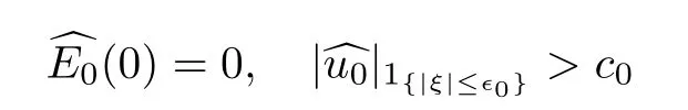
for some constants∈0>0 andc0>0,so there exist two positive constants,C >0 andt0>0,such that

for anyt >t0.

For the low frequency parts,due to Taylor’s expansion,we have that

Due to Parseval’s equality
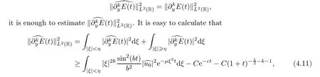
whereηis a small but fixed constant.By a direct computation,we get that

Applying the mean value formula,we have that
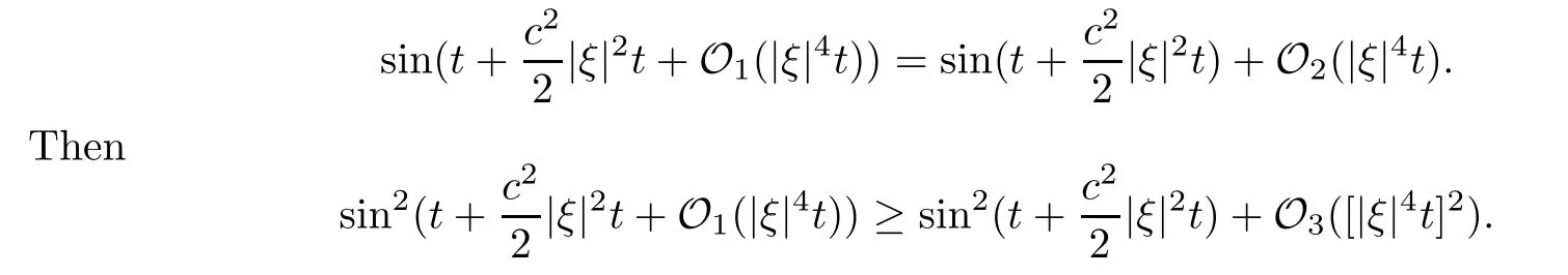
We substitute the above inequality into (5.2) and get that
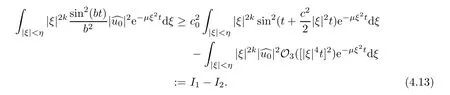
A direct computation gives rise to

It is easy to verify thatH(t) is a continuous periodic function oftwith the periodπ.To achieve our goal,we need to prove the uniform below bound ofH(t) fort >t0witht0>0 being some fixed large time,so we have that
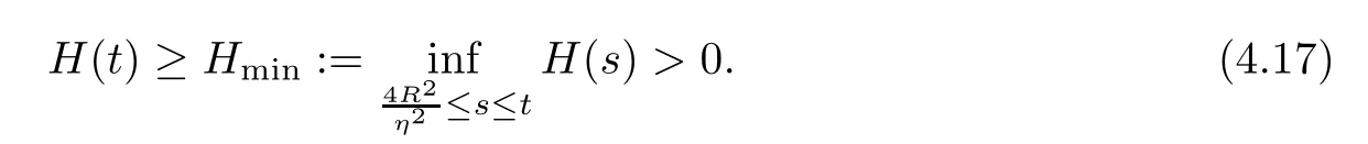
Indeed,it is trivial to note that,for any,there is an integerk0>0 such thatt∈[k0π,(k0+1)π].Thus,to show (4.17),it is sufficient to deal withF(t) in one time periodic domain,namely,t∈[k0π,(k0+1)π] for somek0>0,and

Thus,it follows from (4.15)–(4.18) that

wherec2andc3are some fixed positive constants.Combining (4.13)–(4.14) and (4.19),we can get the below bound of the time decay rates forwith some fixed positive constantc1.Similarly,we can get the below bound of the time decay rate foruwith some fixed positive constantc4. □
4.4 Reformulation of the original problem
Let us reformulate the nonlinear system (2.11)–(2.14) for (E,u).The IVP for (E,u) is expressed as
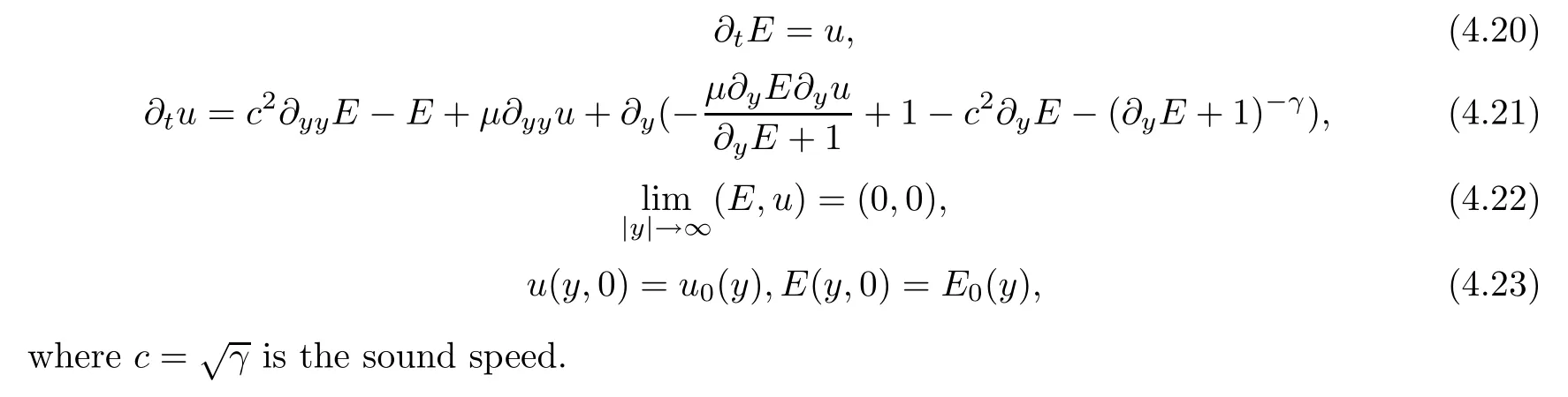

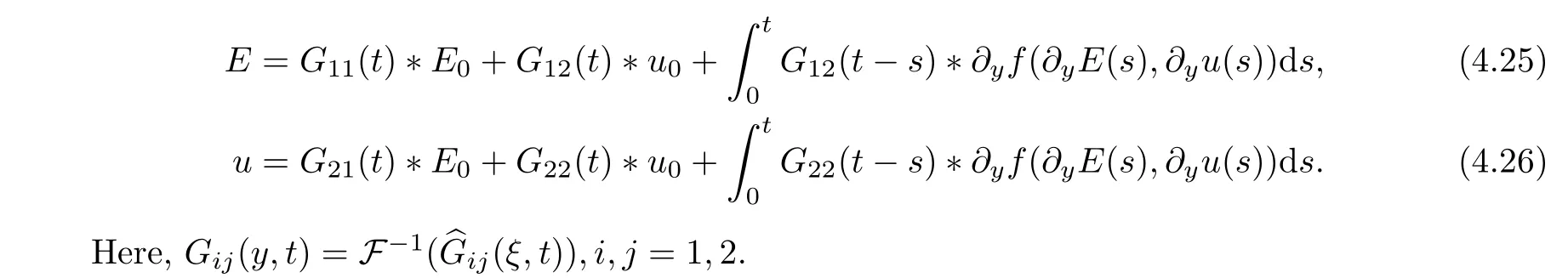
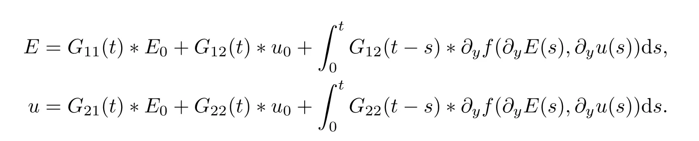
the form of (4.20)–(4.23) is equivalent to the expression

where the differential operatorA(∂y) is defined by (4.6).Thus,due to Duhamel’s principle,we can represent the solutionU(t) in terms of the semigroupS(t) as
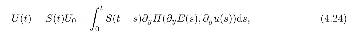
where the semigroupS(t) defined via a multiplier through the Fourier transform is

By (4.10) and (4.24),we have the following two formulas:
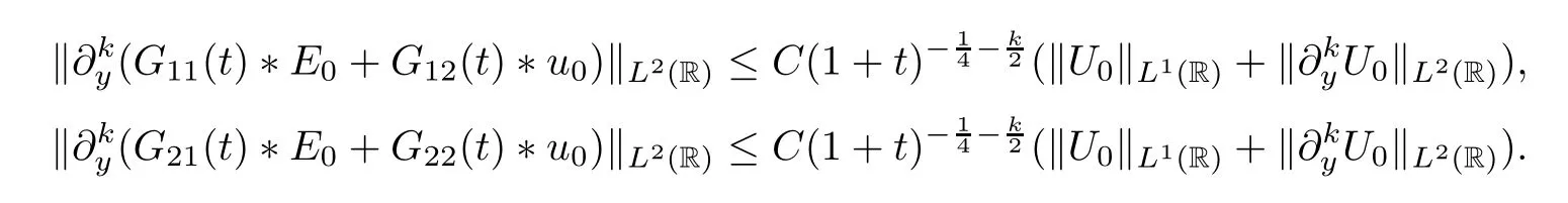
By Proposition 4.1,we have the followingL2-time decay rates for the linear parts:
The following lemma implies thatG12(y,t) plays an important role in closing the energy(4.27) with the time weight in the next section:
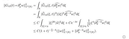
Lemma 4.4Assuming thatw∈H2(R) ∩L1(R),we have that
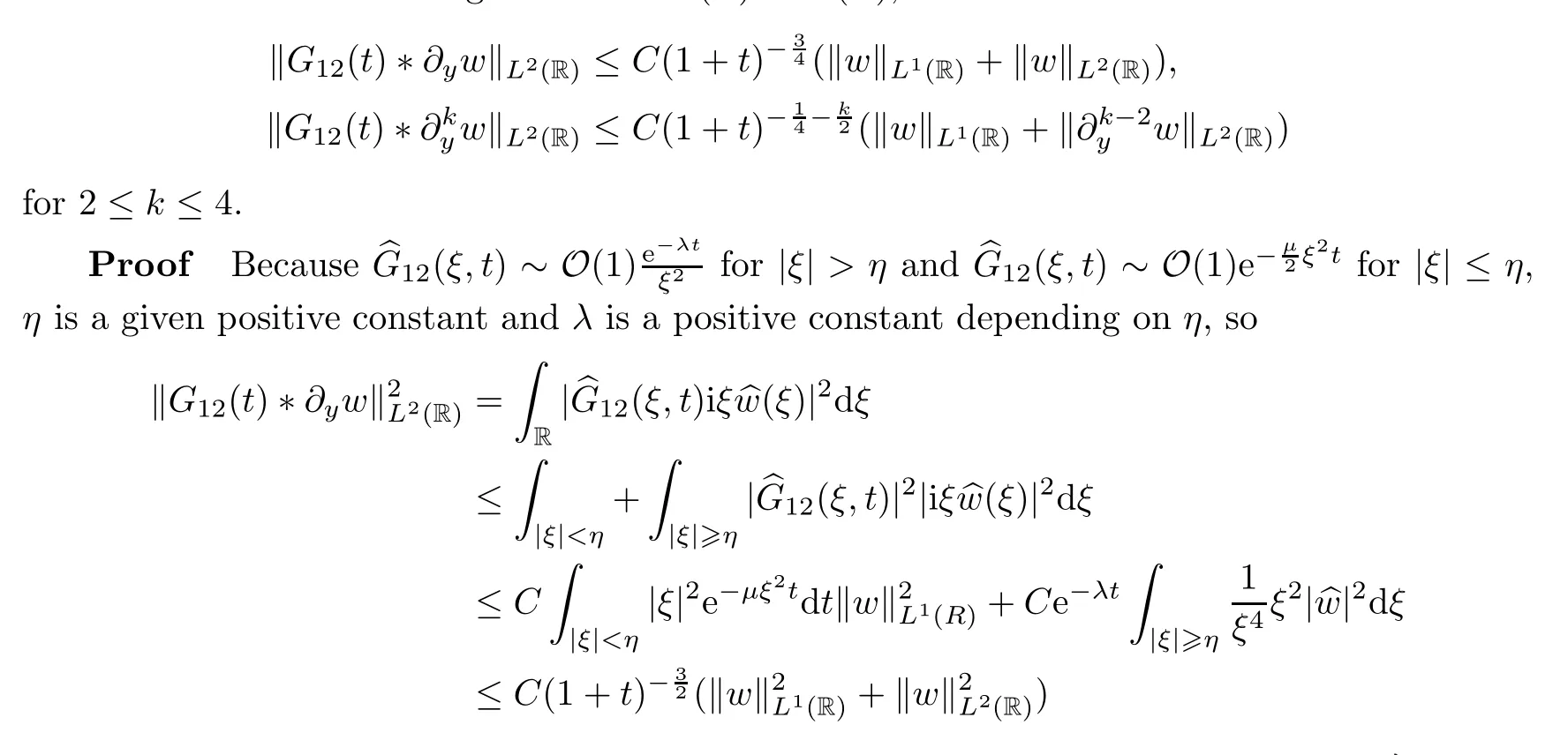
for 2 ≤k≤4,and we have that
4.5 L2-time decay rates for nonlinear system
Lemma 4.5Under the assumption that
for some constantδ1>0 small enough,the solution (E,u) to the IVP (4.20)–(4.23) satisfies that
ProofSuppose that (E(t),u(t)) ∈H4(R) ×H3(R) corresponds to the classical solutions to the IVP (4.20)–(4.23).Assume that the energy with the time weight of (E,u) is expressed as
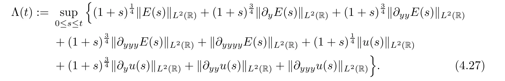
We claim that it holds for anyt≥0 that

the claim (4.28),together with the smallness assumption onδ1,are sufficient to prove this lemma.
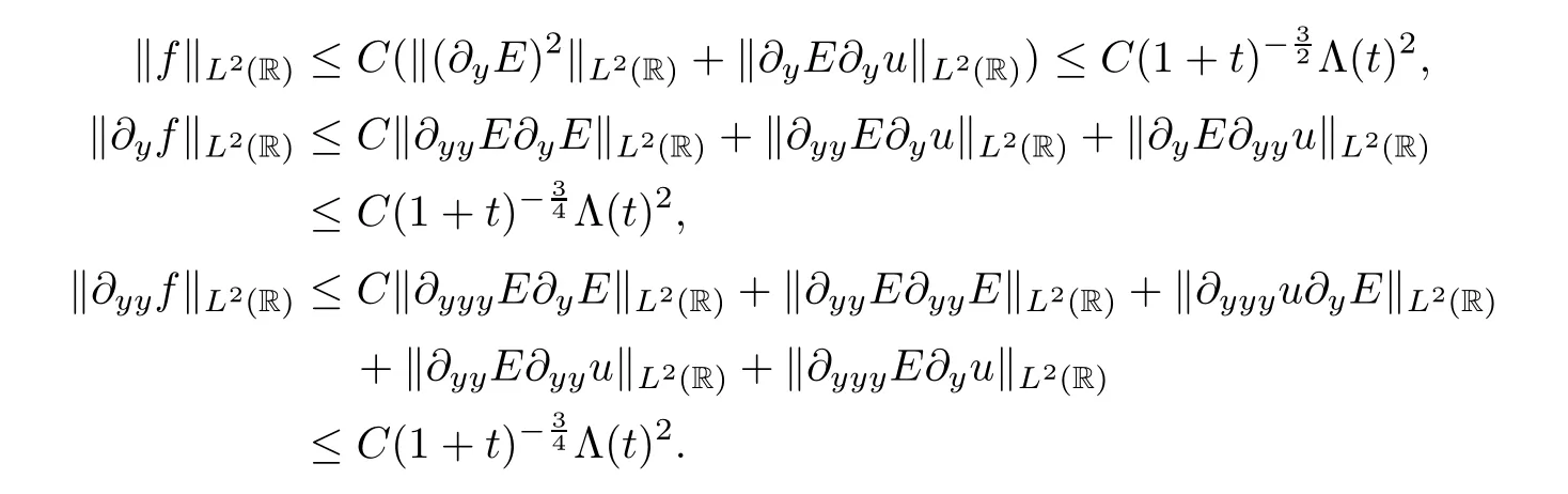
Next,some necessary estimates will be obtained.By Hlder’s inequality and the embedding inequality (3.15),we can get that

For 0 ≤k≤3,with respect to the low frequency parts,we have that
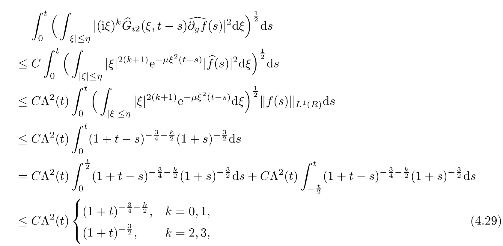
wherek=1,2.
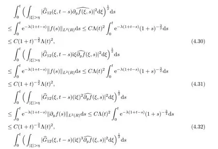
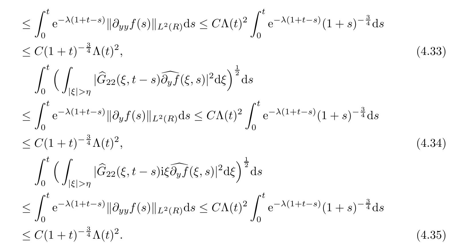
With regard to the high frequency parts,due to Lemma 4.4,we have following estimates:
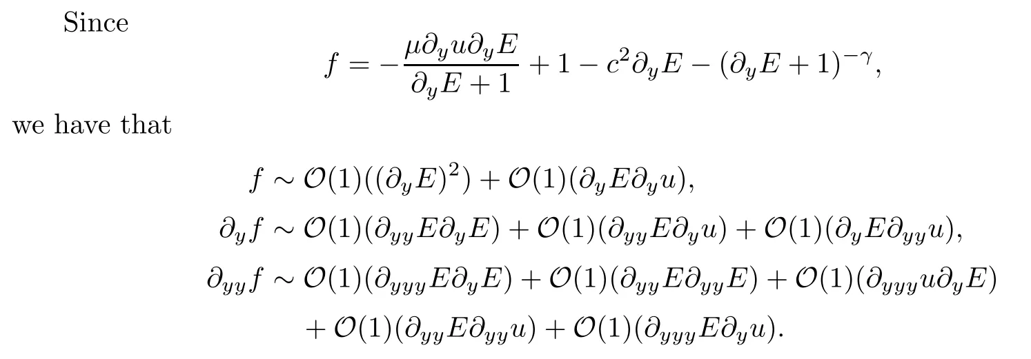
According to the previous computation (4.25)–(4.26),the solution (E,u) can be expressed as
Now,combining (4.29)–(4.35),we can show the main conclusions:

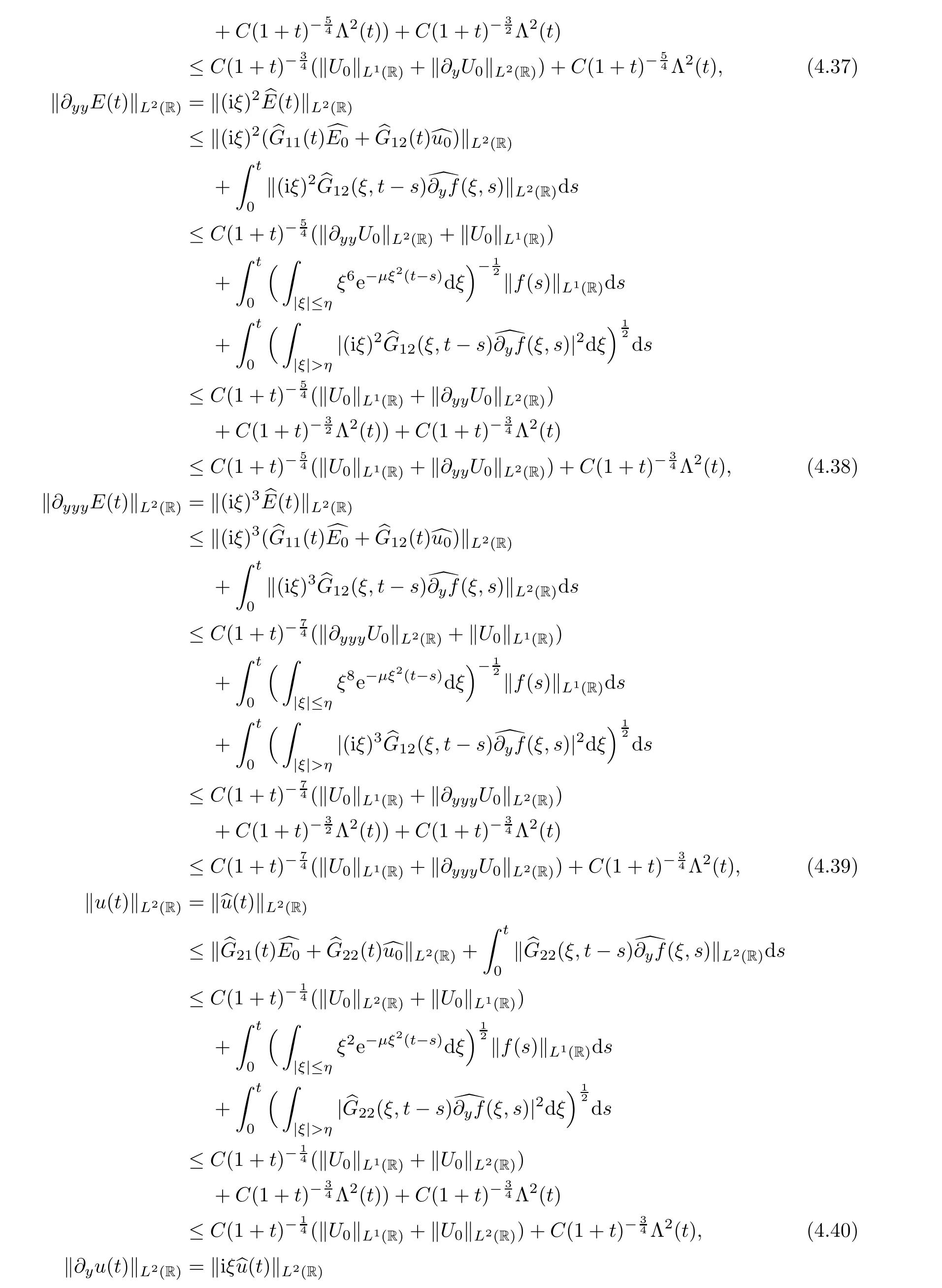
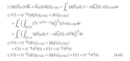
Combining (4.36)–(4.41) and (3.1),we finally obtain that

Thanks to the smallness ofδ1and (4.42),the proof is completed. □
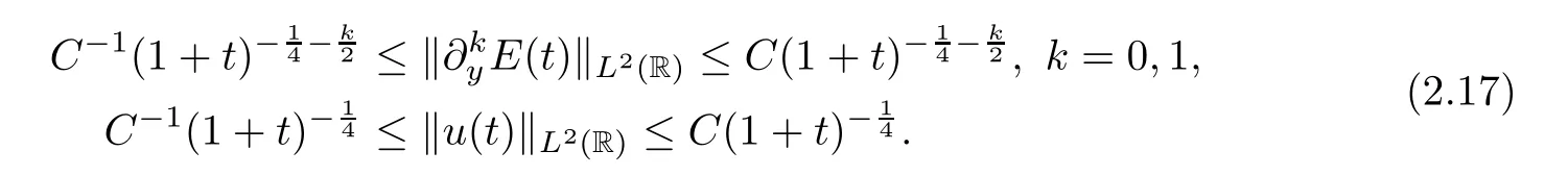
Proof of Theorem 2.2TheL2-time decay rates (2.15) of the solutions (E,u) to the IVP (2.11)–(2.14) have been proven in Lemma 4.5.Fork=0,1,from Lemma 4.5,theL2norm of the nonlinear partsdsof the electric fieldcan be controlled by,which are faster than theL2-time decay ratesof the linear parts of the electric field∂kyE.Then,for anyt >t0,witht0>0 being a sufficiently large time,combining Lemma 4.3 and Lemma 4.5,there exists a positive constantCsuch that,which implies that theL2-time decay rates of the electric fieldare optimal fork=0,1.The proof of the optimalL2-time decay rate of the velocityuis similar to the proof of the electric fieldE,and so is omitted here.Thus,we obtain the optimalL2-time decay rates (2.17) of the solution (E,u) to the IVP (2.11)–(2.14).In this way,we prove that the solutions to the CNSP system converge to those of corresponding linearized system in theL2norm as time tends to infinity,and the proof of Theorem 2.2 is complete. □
5 Time-space Pointwise Behaviors
In this section,we aim to show the time-space pointwise behaviors of the solutions to the IVP (2.11)–(2.14).We first estimate the Green’s function of the linearized system in Subsection 5.1,then we show in Subsection 5.2 that the solutions to the IVP (2.11)–(2.14) are close to a diffusion profile pointwisely,as time goes to infinity.
To begin with,we give some useful lemmas;the first two lemmas were proved in [31].
Lemma 5.1(1) Whenτ∈[0,t] anda2≥t+1,for any positive constantλ,we have that

(2) Whena2≤t+1,we have that

(3) Whenn1,andn3=min{n1,n2},we have that

Lemma 5.2If there exists a constantb >0 such that(ξ,t) satisfies that

for any nonnegative integerα,βwithβ≤2N(N >r >),then
whereκand m are any fixed nonnegative integers,a+=max{0,a} and
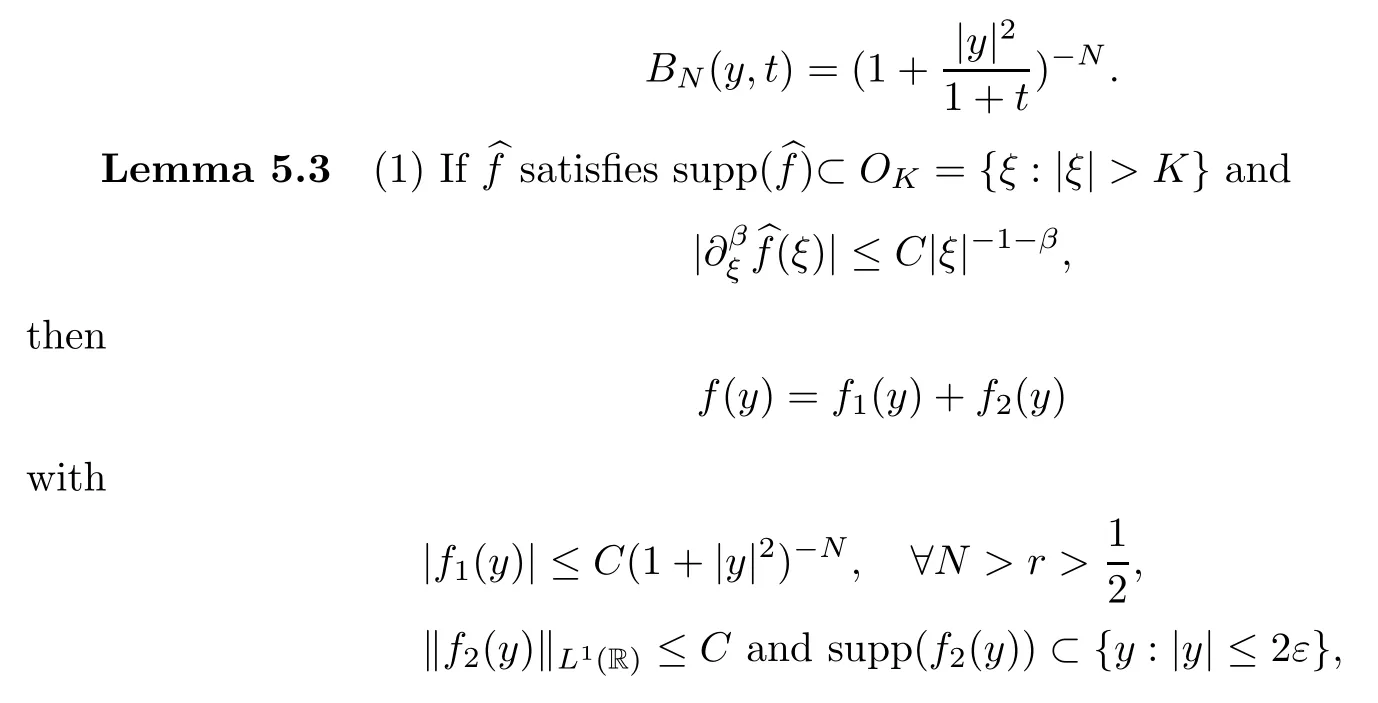
whereεis a small constant.
for someK >0,then,for anyN >r >,

whereδ(y) is the Dirac measure.
Proof(1) Define the smooth cutofffunctionχ(y) which satisfies that
for some small constantε.We dividef(y) intof1(y) andf2(y),which satisfy
For anyβ≥2N >2r >1,since
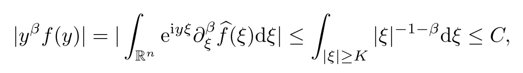
it is implied that

Forf2(y),we have that

where the third equality holds thanks to Parseval’s inequality,the fourth equality holds thanks to the equalitythe fifth inequality holds thanks to a convolution type Young’s inequality,and the last inequality holds because 1 -χ(y) is a rapidly decreasing function and the Fourier transform is a bijection in the space of the rapidly decreasing function.

It is necessary to prove the following useful inequalities to estimate the nonlinear terms:
Lemma 5.4(1)

whereα=0,1 andN >r >.
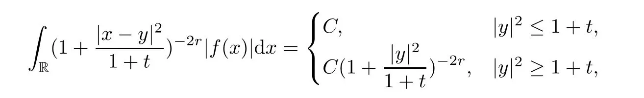
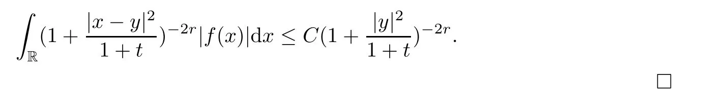
(2) Assume that supp(f(y)) ⊂{y: |y| ≤2ε},withεbeing a small constant and ‖f‖L1(R)≤C.Then we have that

wherer >.
Proof(1) When |y|2≤1 +t,due to (2) of Lemma 5.1,we have that
When |y|2≥t+1,since
by (2) of Lemma 5.1,we have that
(2) Since
and due to (2) of Lemma 5.1,we have that
5.1 Pointwise estimates of Green’s function
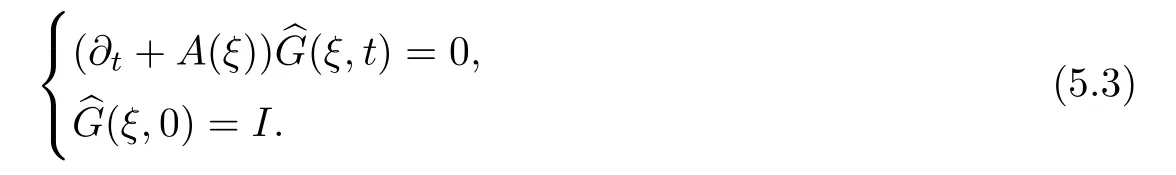
We consider the Green’s function for the linearized system (4.5):
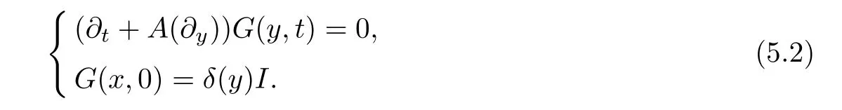
Here,δ(y) is the Dirac measure andIdenotes the 2×2 unit matrix,and the symbols of operatorA(∂y) are
For (5.2),after the Fourier transform,we obtain that
By direct calculations,we get that
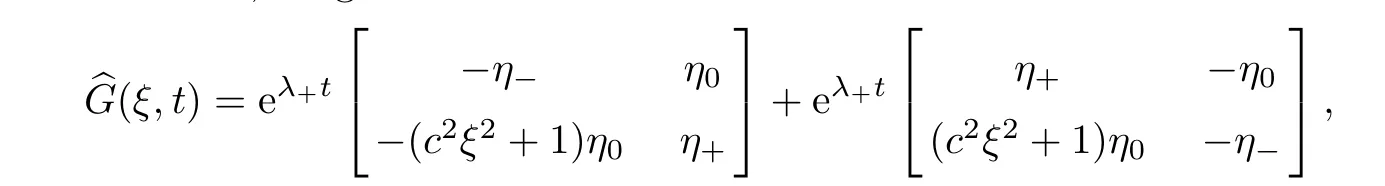
whereη0(ξ)=(λ+(ξ)-λ-(ξ))-1,η+=λ+(ξ)η0(ξ),η-(ξ)=λ-(ξ)η0(ξ) andλ±(ξ) are defined by (4.9).

be smooth cutofffunctions,where 2∈<K.Setχ2(ξ)=1 -χ1(ξ) -χ3(ξ) and
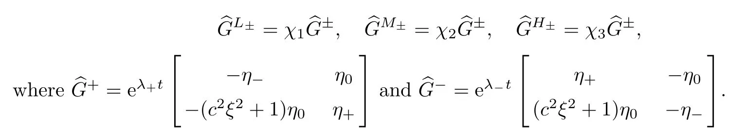
We consider the low frequency parts of the Green’s function.We denote each term at the low frequency parts by,wherei,j=1,2.The pointwise estimates of each term will be given.
For |ξ| ≤2ε,we have that
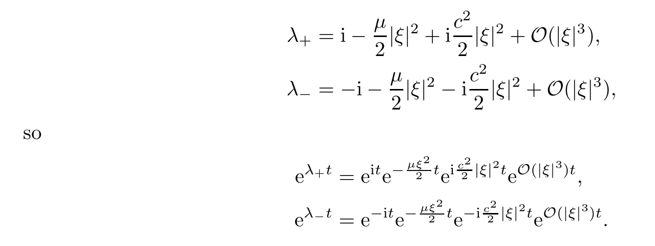
Furthermore,we have that

Thus,we get that
Lemma 5.5Assume that |ξ| ≤2ε.Then there exists a constantb >0 such that

wherei,j=1,2.
ProofBy differentiating both sides ofwith respect toξ,we immediately obtain(5.4). □
Proposition 5.6For sufficiently smallε,we have that

wherei,j=1,2 andN >r >.
ProofThanks to Lemma (5.2) and Lemma (5.5),we directly obtain (5.5),and the proof is completed. □
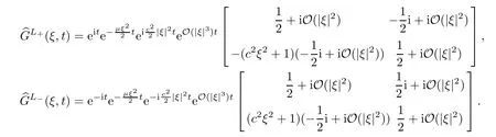
Proposition 5.7Assume that some fixed constantsε >0 andK >0 satisfyε <Then there exist two positive constants b and C such that
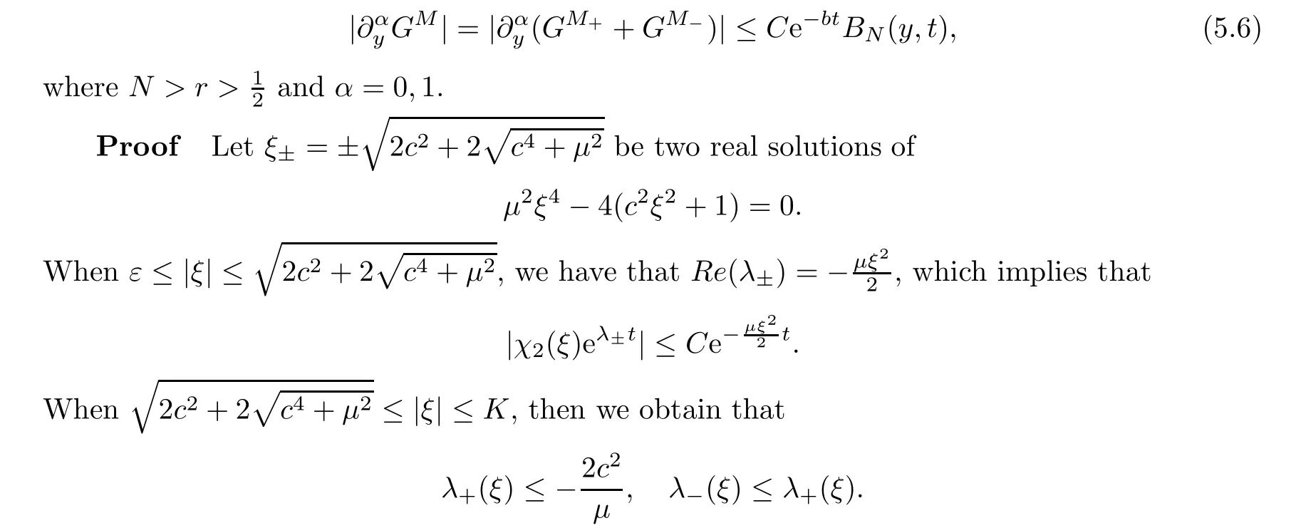
Thus,we have that
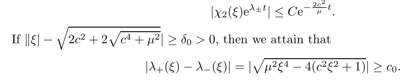
Thus,for some fixedd >0,we have that
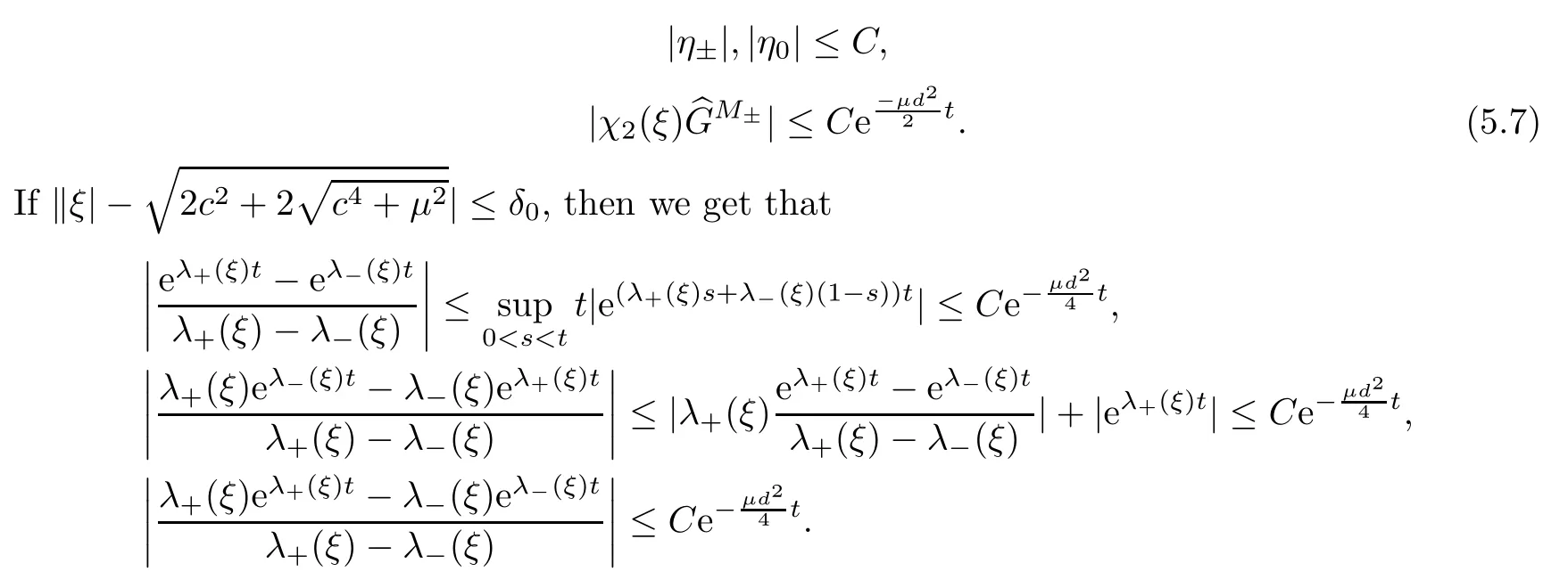
Thus,for any fixed∈andK,we have that

Now,we give the estimates ofby induction onβ.Suppose that 0 ≤β≤l-1.Then it holds that

which is true whenβ=0 by (5.7).From (5.3),we have that
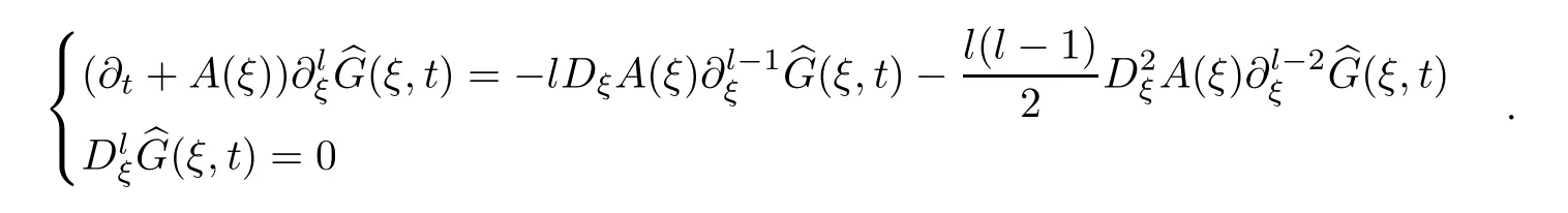
Hence,forβ=l,we have that

which implies that

for 1 ≤β≤l.By using (5.8) when |y|2≤1 +t,using (5.9) when |y|2≥1 +t,and using the fact that

for some constantθ.By the Lemma 5.2,we complete the proof. □
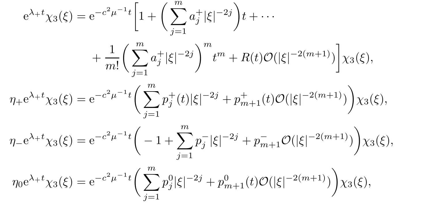
Thus,we find that
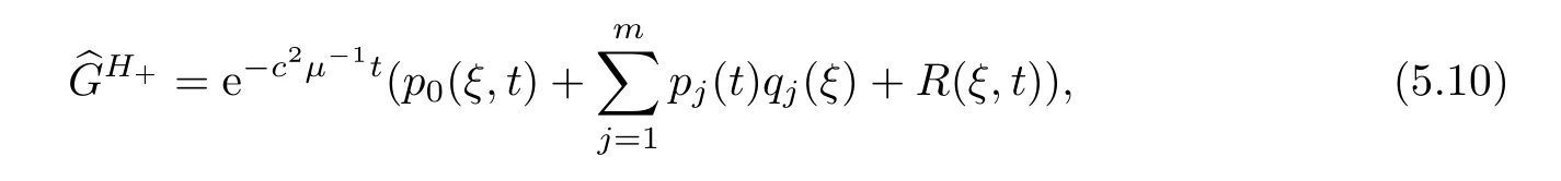
wherep0,qj(j=1,2,···,m) are matrices which satisfy that

As in [11],by Lemma 5.3,we can divide F-1(|ξ|-2jχ3(ξ)) into two parts,

whereεis sufficiently small.

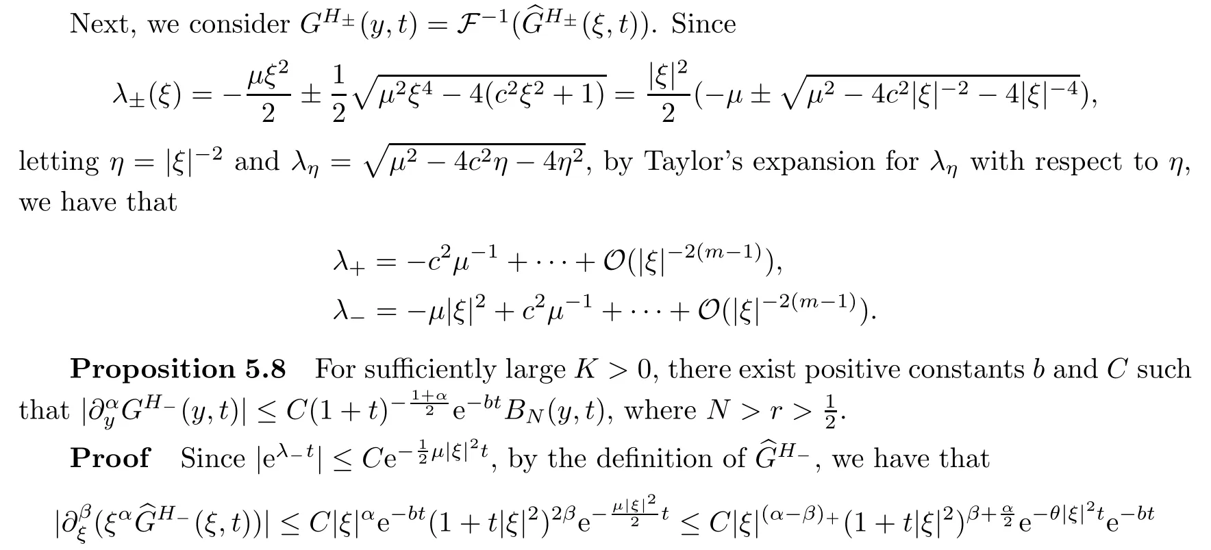
where |f0(y)| ≤(1 +y2)-NandN >r >.By the definitions ofGH+andLj,we have the following proposition:
Proposition 5.9For sufficiently largeK,there exists a distribution
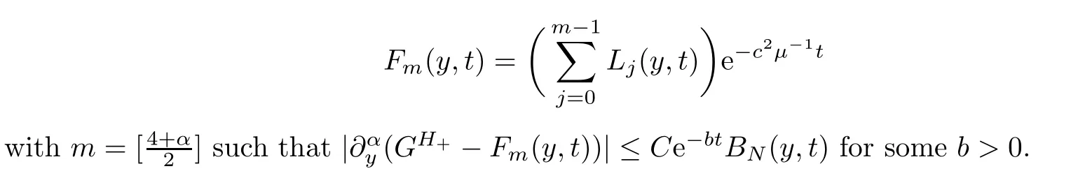
Theorem 5.10For anyy∈R andt >0,we have that

Remark 5.11Proposition 5.6,Proposition 5.7,Proposition 5.8,Proposition 5.9 and Theorem 5.10 imply that the time decay rates of the Green’s function are determined by the lower frequency parts;this plays an important role in the pointwise estimates of the solutions for the nonlinear system in the next section.
5.2 Pointwise estimates of nonlinear system
For the solutionU=(E,u)⊤to the IVP for original system (4.20)–(4.23),from (4.25)–(4.26),we have that
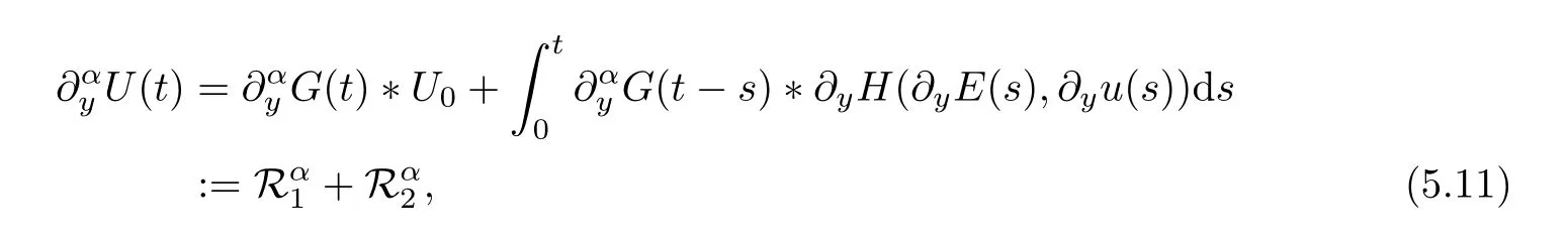
whereU0=(E0,u0)⊤.We should admitα=0,1 for the rest of paper and set that
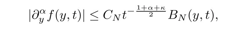
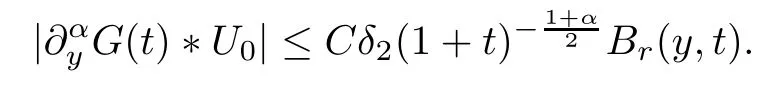
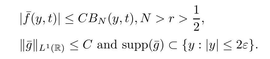
Lemma 5.12Suppose that the initial dataU0=(E0,u0)⊤satisfies that|y|2)-r,whereδ2>0 is a constant small enough andThen
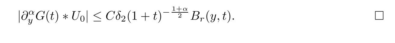
ProofWe divideinto three parts:

By (3) of Lemma 5.1 and Theorem 5.10,we have that
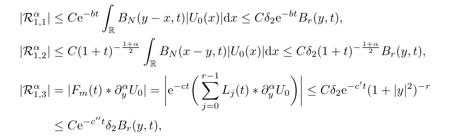
wherec′′<c′<c.Combining the above three inequalities,we get that
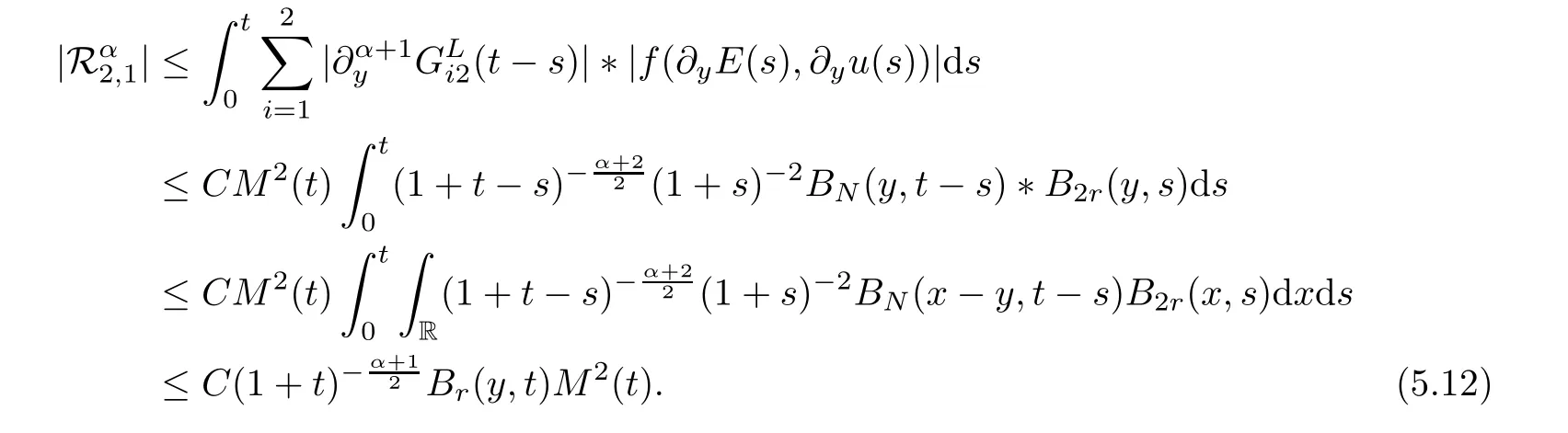
Next,we consider the nonlinear termsin (5.11).Integrating by parts,we have that
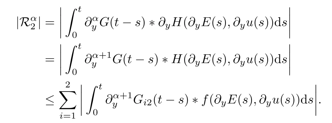
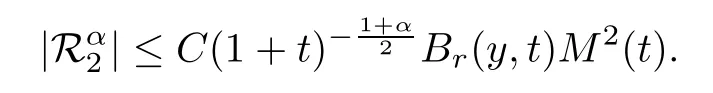
Lemma 5.13For the nonlinear partsin (5.11),we have that
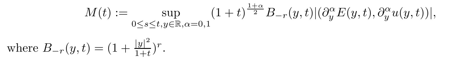
ProofBy the definition ofM(t),we have that

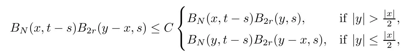
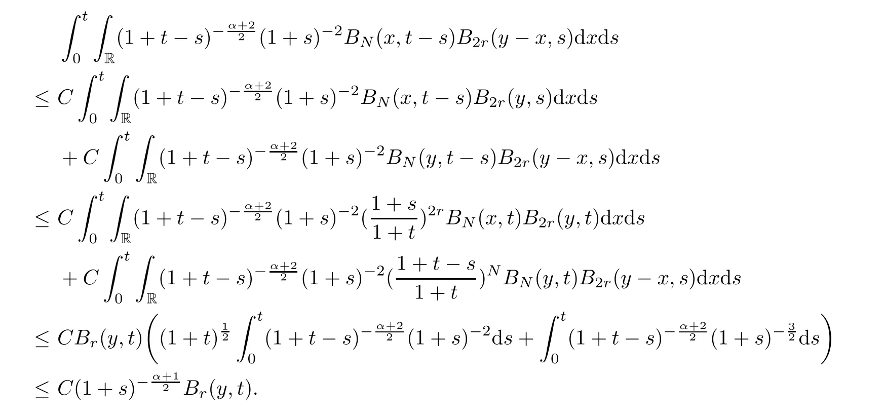
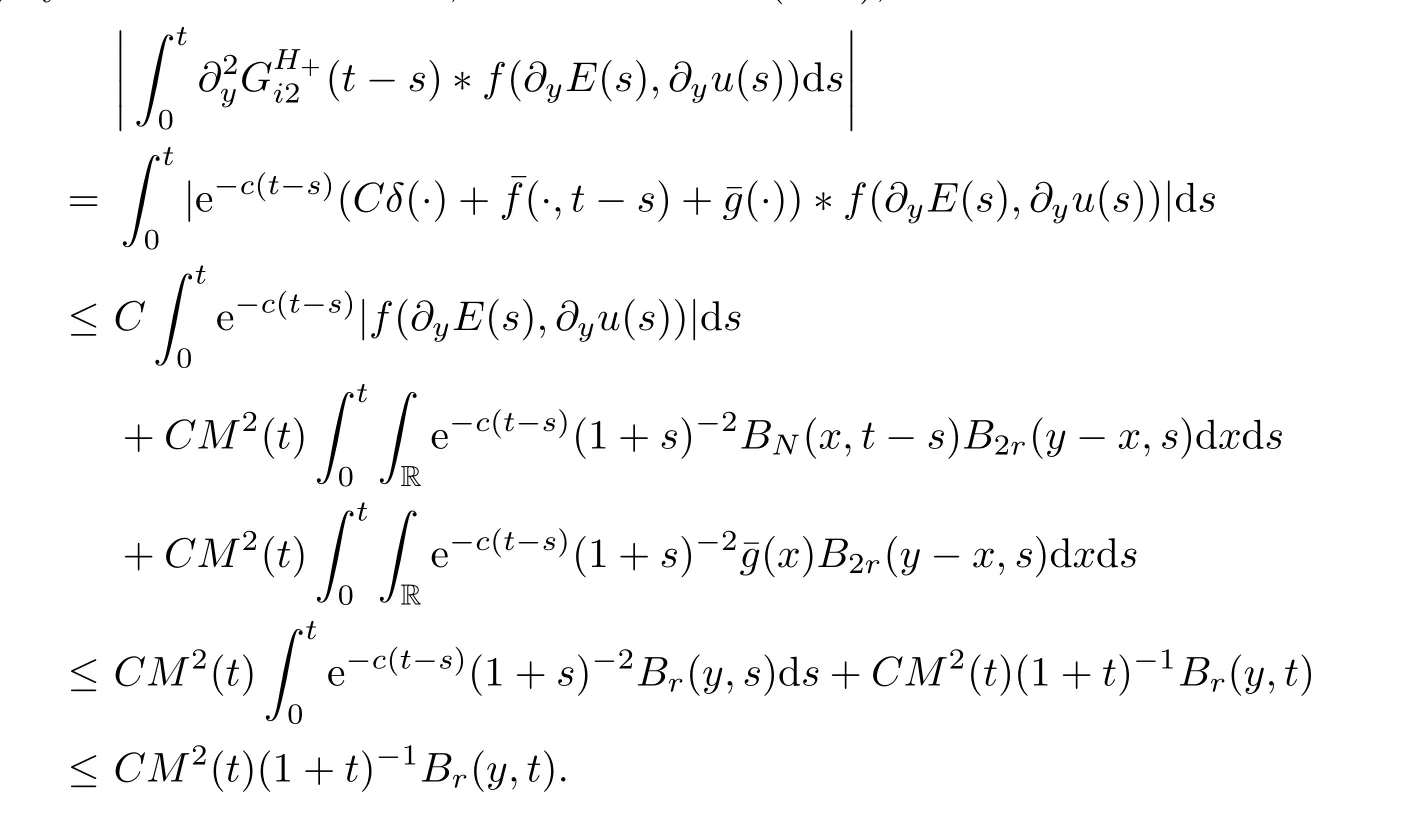
In order to estimate the nonlinear parts,is divided into four parts:

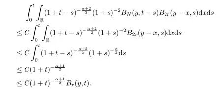
From Lemma 5.4 and Proposition 5.6,we have that
Similarly,owing to Proposition 5.7 and Proposition 5.8,we obtain that

wherej=2,3.
For the high frequency parts,from (5.6),we have that

By Lemma 5.3,we get that

where
Making use of Lemma 5.1,Lemma 5.4,and (5.14),then it holds that

Similarly,by virtue of Lemma 5.1,Lemma 5.4 and (5.15),we have that
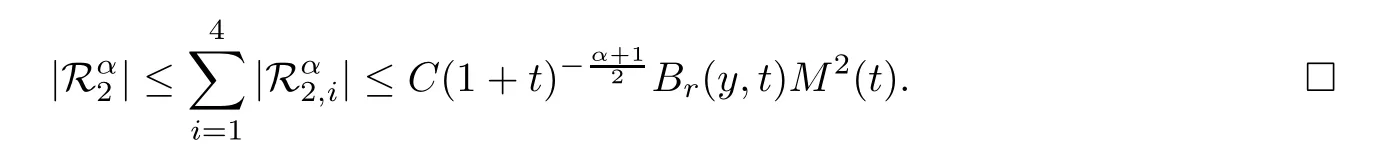
The above two inequalities imply that

Therefore,combining (5.12),(5.13) and (5.16),we have that
Proof of Theorem 2.4By means of Lemma 5.12 and Lemma 5.13,we have that

Since we assume thatδ2>0 is sufficiently small,by the continuity ofM(t),M(t) ≤Cδ2.The proof of Theorem 2.4 is therefore complete. □
AcknowledgementsThe authors would like to thank Professor Hai-Liang Li for helpful discussions and comments.
杂志排行
Acta Mathematica Scientia(English Series)的其它文章
- RELAXED INERTIAL METHODS FOR SOLVING SPLIT VARIATIONAL INEQUALITY PROBLEMS WITHOUT PRODUCT SPACE FORMULATION*
- PHASE PORTRAITS OF THE LESLIE-GOWER SYSTEM*
- A GROUND STATE SOLUTION TO THE CHERN-SIMONS-SCHRÖDINGER SYSTEM*
- ITERATIVE METHODS FOR OBTAINING AN INFINITE FAMILY OF STRICT PSEUDO-CONTRACTIONS IN BANACH SPACES*
- A NON-LOCAL DIFFUSION EQUATION FOR NOISE REMOVAL*
- BLOW-UP IN A FRACTIONAL LAPLACIAN MUTUALISTIC MODEL WITH NEUMANN BOUNDARY CONDITIONS*