RAO Y N, BAARTMAN R

(TRIUMF, 4004 Wesbrook Mall, Vancouver British Columbia, V6T2A3, Canada)

Abstract: Knowledge of the phase space density distribution in details is useful to understand subsequent evolution of the charged particle beam in a transport line. This makes the beam tomography very useful in the application for beam diagnostics. This application is not limited by the beam energy, as opposed to the emittance scanner. This paper presented the simulations and measurements we undertook in TRIUMF beam-lines to validate the maximum entropy (MENT) technique for the tomographic reconstruction of beam density distribution in the 2-dimensional transverse phase space. Beam profiles were taken with a single wire scanner while changing an upstream quadrupole’s strength. Moreover, the phase space plots were directly measured with emittance scanner. A close comparison was made on the resulting phase space density distribution and the emittance value at the same location of the beam-line. They show good agreement.

Key words：beam tomography; maximum entropy algorithm; phase space; emittance

The tomography is a process of estimating an unknown higher dimensional density distribution from a set of projections measured in a lower dimensional subspace at various observation angles[1]. There are several algorithms available to reconstruct the tomography from projection data, such as the algebraic reconstruction technique (ART)[2], filtered back-projection algorithm (FBP)[3], and maximum entropy (MENT) algorithm[4], etc. In the absence of large number of projections (views), the MENT algorithm can reconstruct a density distribution that maximizes the entropy and simultaneously reproduces all the measured projections exactly, making it very useful for application in accelerator beam diagnostics[5-6]. In combinatorial theorem, the entropy is interpreted as a measure of the number of arrangements (i.e. multiplicity) in a system to form a certain distribution. For an ensemble of a large number of particles, the most probable distribution is the one which is most easily produced by nature, i.e. the distribution with maximum entropy, and in the mean time coincides with the measured projection profiles, as it contains everything we know, nothing else. Usually the particle beam distributions are smooth, possess only moderate amounts of asymmetry, and are available for measurement at only a limited number of views, typically in the order of 10 instead of 100. The MENT algorithm does not assume any prior knowledge of the distribution. It however does assume that the motion of particles completely follows a linear mapping, represented by a transfer matrix. This matrix depicts a geometrical transformation of the phase space, usually a combination of rotation and stretch. The geometrical connection means that a projection of the phase space at the observation location(s) is related to the projection of the phase space at the source location in certain rotated direction. This rotation angle is governed by the focusing strength(s) of optical element(s) in between. This is to say, the tomographic technique involves measuring beam projections under various rotation angles of the phase space, related by arbitrary linear transformations. Specifically, the beam profiles are measured with either multiple or a single monitor(s) (e.g. wire scanner or view screen) in a beam-line, while varying the excitation (voltage or current set-ting) of an upstream optical element such as a quadrupole or solenoid. The reconstruction is therefore realized at a location in front of the optical element being scanned. Such an application is not limited by the beam energy. Mathematically, the MENT algorithm is reviewed using a simple continuum derivation of the factored product form for the maximum entropy reconstruction function. An iterative procedure is employed to solve a large system of coupled non-linear integral equations that result when the product form is substituted into the projection integral constraints[7]. The MENT technique has been used in the accelerator physics community[8], including LANL[9], ITAM[10], DESY[11-12], PITZ[13-14], TRIUMF[15-16], Daresbury Laboratory[17-18], PSI and SNS[19], to beams without space charge and recently applied to electron beam with space charge[18-20]by assuming linear forces. However, vast majority of the published work on the beam tomographic reconstruction are either using a phantom i.e. completely hypothetical distributions, or using distributions that are simulated with particle tracking code (e.g. ASTRA). Our studies focus on the MENT technique, not the FBP at all, because we only need to use ～10 projection profiles for the reconstruction, instead of >100 as imposed by the FBP algorithm[18,20]. And we’ve not only used the simulations but also used the experimental measurements to validate the MENT technique. The novelty of our work is that we’ve directly measured the phase space density plot with emittance scanner to compare with and therefore verify the MENT reconstructed results. To the best of our knowledge, there has been no report yet on such examination. Moreover, we discovered from our studies that in order to minimize distortion and error in the MENT reconstruction, the phase space rotation angle must be made larger than 90°. This is to say, a minimum beam size must be reached and covered at the location of beam profile monitor over the scan range of the optical element(s). Such a criterion is easy to quantify in practical applications of MENT. We conclude that this is the key point for a minimized error in the MENT application, as opposed to Daresbury Laboratory’s claim[17-18]about the necessity of equal rotation angle intervals. We present details of these simulations and measurements in Sections 2 and 3 after reviewing the basic principle of phase space tomography in Section 1.

1 Tomography algorithms

We briefly summarize the basic principle of phase space tomography[3,21], with intention to give insights into the nature of the methods. This will be using two-dimensional distribution as an example, with goal to derive a formula to calculate a source distributionf(x0,x′0) from its projectionsP(x) in the real space, given by:

(1)

where the point (x,x′) corresponds to the point (x0,x′0) following a linear transformation. This transformation is similar to a geometrical rotation in the Cartesian frame involving a scaling factor and a rotation angle.

The algorithms that have been used to compute the tomographic reconstructions include the FBP[3], ART[2], and MENT[4], etc. In the FBP theory, the source functionf(x0,x′0) is restored by back-projecting the filtered version of the projections and is represented as[3]:

f(x0,x′0)=

(2)

whereF(w,θ) is the two-dimensional Fourier transform of the object functionf(x0,x′0), and it is just the one-dimensional Fourier transformFθ(w) of the source function’s projection at angleθ;wis the frequency;sis the scaling factor.

Both the scaling factorsand the angleθof the projection are calculated from the beam-line transfer matrix[21]. Eq.(2) indicates that the FBP algorithm requires the projection angleθto be covering a full range of 180°. As such, in practical applications a large number of projections have to be taken, typically above 100[18,20]. But limited by the beam-line optics and the profile monitor’s placement, usually only small number of projections (typically 10) are available from the actual measurements, and also the projection angle does not span over the entire range of 180°. In such circumstances, the FBP algorithm produces streaking artifacts[14,17]and consequently falsify the result as the inversion is not unique. This is a severe problem of FBP algorithm when the number of views is small.

In contrast, the MENT algorithm[4,9]performs better. It produces a maximum entropy solution without the streaking artifacts. The entropy is defined as a measure of the multiplicity of a system. For the distribution functionf(x0,x′0), the entropy is represented as:

(3)

For a system of a large number of particles, the most probable distribution will be that one of a maximum entropy i.e. of the greatest multiplicity[4], because it is maximally noncommittal about unmeasured parameters. So, taking into account the projections prescribed by Eq.(1) as boundary conditions, followed by applying a stationary condition ∂E(f)/∂f=0, one finds a simple product form for the source function:

(4)

where each of the unknown functionsHi(xi)(i=1,2,…,I) has only one argumentxi, completely specified by the corresponding linear transformation between the source location of subscript 0 and the observation location(s) down the beam-line, while their shapes are to be determined by fitting the projection data. So, the task is merely to find theseH-values.

Substitution of Eq.(4) into the projection constraint Eq.(1) for all theIprojections results in a set ofIsimulta-neous nonlinear equations to be solved for theIunknown one-dimensional functionsHi(xi), expressed as:

k=1,2,…,I

(5)

Since the mapping is simply identity fori=k, one can factorHk(xk) out of the constraint integral for thekthview, and write:

Pk(xk)=Hk(xk)Qk(xk)

(6)

Since the projection profiles Eq.(1) are treated as boundary conditions in the MENT algorithm, all the input profiles must be exactly reproduced from the resulting tomography. If any of them appears not, then it means that this is bad data and must be corrected or even discarded if it’s not correctable. The good profiles are meant those ones that are sampled under the same beam current and under the same beam conditions. This can be quantified for a judgement based on the linear optics. The linear optics is the physics that one can rely on, because a linear and uncoupled transport system between the source location and the observation location(s) is the only assumption that is made in the MENT algorithm. This means that square of the rms beam sizes obtained from the measured profiles must follow a parabolic dependence of the focusing strength of the optical element being scanned. Our investigations in the following sections manifest the importance of this rule.

2 Simulations

MENT is the technique used for the tomographic studies in this paper. Typically, we only need to use the order of 10 projection profiles for the reconstruction, instead of 100 as used in the FBP algorithm[18,20]. A series of simulations have been carried out to determine its performance using simulated distributions. To map the beam phase space, we use the method of quadrupole scan or solenoid scan. The beam profile and size at a given location downstream from the scanned optical element are measured as a function of its focusing strength.

2.1 Quadrupole scan

This research is dedicated for the TRIUMF injection beam-line[16], where a front-end electrostatic quadrupole was scanned between -10 kV and +10 kV in a step of about 1 kV, creating 22 data sets of projection profiles available for the reconstruction.Fig.1 compares the MENT reconstructed tomography and the original distribution, along with the statistical values (2rms) of the beam size, divergence and emittance which are calculated from the phase space density distributions. Similarly hereinafter.

It’s seen that the reconstructed result closely agrees with the original one, not only on the crescent shape but also on the statistical values of the beam size, divergence and emittance. There are 22 projection profiles available in the whole data set. An interesting question was raised: How small a subset of the data can be used to reproduce the peculiar crescent shape? The answer is that a subset of voltage setting ≥0 kV can, while the subset of voltage ≤0 kV can not. This is because the former subset can make the phase space rotation larger than 90° so that the projections observed at the monitor are informative enough for a good reconstruction; while in the latter case, the rotation angle is much smaller than 90°. This is illustrated in Fig.2, Where three particles are marked, showing that the rotation angle exceeds 90° over the entire range of the quad scan between -10 kV and 10 kV.

Fig.1 Original phase space (left) and MENT reconstructed tomography (right)

Fig.3 shows the results reconstructed using different subsets of the data. In comparison with the original picture shown in Fig.1,Fig.3a is completely distorted and disagreed,Fig.3b is not good enough in terms of the shape, while Fig.3c and Fig.3d are very well reproduced and agreed. Notice that an elliptical-shaped phase space tends to be produced but in fact it’s a significantly distorted result; both the shape and the statistical values disagree with the original ones (Fig.3a). This happens when using the 12 sets ofV≤0 kV data. Nevertheless, the 12 projection profiles still get well reproduced (nearly as good as using all the 22 sets of data), implying that the solution is not unique. Besides, it’s seen from Fig.3b, c and d that under the good condition of rotation angle ≥90°, the more samples one takes, the more accurate result one can achieve from the reconstruction. These samples are not necessarily taken at uniform rotation angles in the phase space, although the quad’s strength is changed in nearly an equal step size.

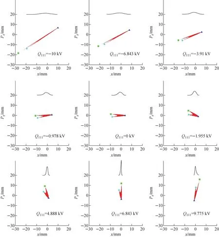
Fig.2 Phase space of identical scale in x and Px=αxx+βxx′ (αx and βx being Twiss functions), visualized at location of profile monitor under various voltage settings of quad, along with projection profiles produced on x axis

a—With all 12 sets of V≤0 kV data;b—With 3 sets of V≥0 kV data (i.e. 0, 4.888 and 9.775 kV); c—With 6 sets of V≥0 kV data (i.e. 0, 1.955, 4.888, 5.865, 7.820 and 9.775 kV);d—With all 11 sets of V≥0 kV data Fig.3 Results reconstructed by using different subsets of quad’s scan data

Fig.4 Square of beam size measured at monitor vs. voltage setting of quad

From each projection profile, one can calculate the beam size (rms). The measure of the rotation angle is reflected in the beam size vs. the quad’s strength. As is shown in Fig.4, the square of beam size vs. the quad’s excitation shows a parabolic dependence, because the linear beam optics followsσ2=Rσ1RT(whereRis the linear transfer matrix from location 1 to location 2 where the beam’sσ-matrices areσ1andσ2respectively). Apparently, the positive voltage side reaches a minimum beam size while the negative side does not. The minimum beam size occurs when the phase space turns upright. This indicates that in practical applications of the MENT technique, the quad’s scan range must be made wide enough to trace out a minimum beam size at the monitor.

This way allows to reconstruct the phase space with reduced distortions and errors especially for a s-shaped or crescent-shaped phase space which can emerge coming out of the ion source. Nevertheless, it’s worthwhile to mention that this condition is not a dictation from the MENT algorithm itself; instead, it is a requirement placed by the measurement errors. Essentially, the tomographic reconstruction procedure is no different from the three-monitor-method or the quad-scan-method[22]that is commonly used for the measurements of beam emittance and Tiwss parameters. Either method does not guarantee automatically a measurement with the desired accuracy. To accurately fit the parameters (emittance and Twiss parameters) one must be able to vary the beam size considerably such that the nonlinear variation of the beam size with quadrupole strength becomes quantitatively significant. The measurement errors can be minimized when variation of the quadrupole strength is changed widely enough to trace out a parabola-like curve for the beam size covering a narrow focal point.

2.2 Solenoid scan

Similarly, the solenoid scan method can be applied for the phase space reconstruction too, and such a reconstruction can be realized for the 2×2D instead of for the full 4D phase space. This requires for a measurement of beam distribution in the 2Dx-yreal space using the view screen. With the 2D measurement, the coupling between the two transverse planes due to the solenoid field can be removed through the coordinate rotation transformation, allowing to simplify the 4D issue into a 2×2D issue.

It’s well known that the 4×4 transfer matrix of a solenoid for the transverse plane is represented as:

(7)

wherec=cos(kLe);s=sin(kLe);k=Bz/(2Bρ) is the focusing strength,BandLeare the field strength and the effective length,Bρis the beam magnetic rigidity.

TheTslcan be decomposed into:

(8)

where theUis the uncoupled matrix while theRis simply a rotation transformation. This means that one can decouple thexplane with theyplane by applying an inverse matrix ofR, i.e.:

(9)

to the beam distribution measured with the view screen. This is to say, just apply the following 2×2 rotation matrix:

(10)

to the coordinates as measured in the (x,y) plane at the view screen.

We demonstrated this method using TRIUMF e-inac front-end as the beamline model[23], where the electrons come out of electron gun, propagate through a solenoid followed by a view screen taking a snapshot in the transverse real plane. For our purpose the initial phase spaces are assumed to be elliptical in the (x,x′) plane and s-shaped in the (y,y′) plane (Fig.5), and fully coupled between the two planes.Fig.6 to Fig.8 show the resulting distributions of the beam under various excita-tions of the solenoid, before and after removing the fore-mentioned coordinate rotation due to the solenoid field, and the red and cyan lines mark the axes, allowing to visualize the rotation angleθrot. The beam projections produced after the rotation removal, along with the calculated transformation matrixU(not theTsl) in either plane, were input for the MENT reconstruction. The results are shown in Fig.9. Apparently, they are exactly reproduced, in comparison with the original pictures as shown in Fig.5. Again, it’s vitally important for the solenoid-monitor combination to scan out a minimum beam size in order to enable the reconstruction with reduced distortions and errors.

Fig.5 Initial phase spaces in (x,x′) and in (y,y′), hypothetical model for solenoid scan method demonstration

Fig.6 Density distribution of beam measured in real space under different field strengths of solenoid, shown before (left) and after (right) coordinate rotation with angle θrot=BsolLe/(2Bρ)

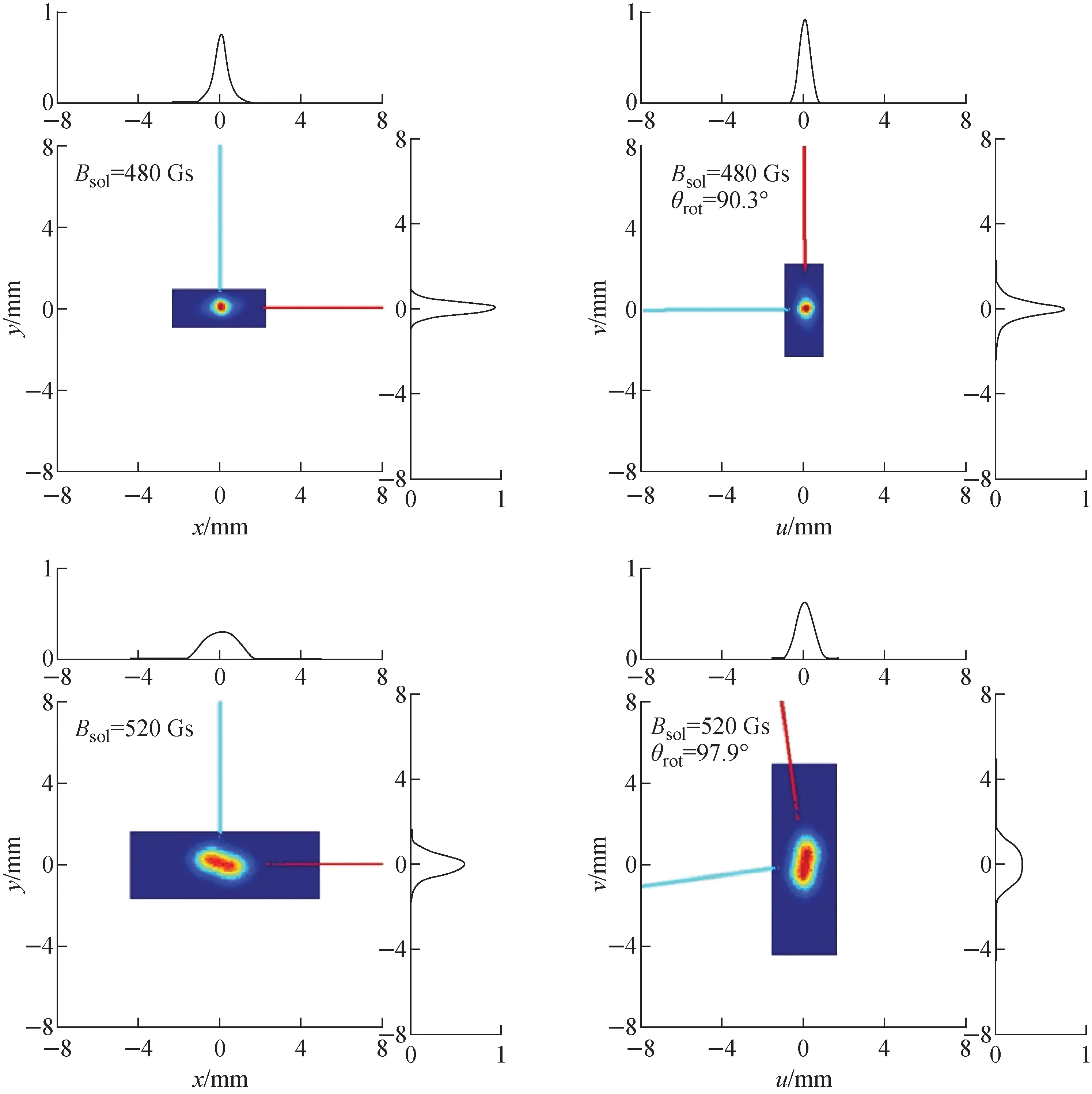
Fig.7 Density distribution of beam measured in real space under different field strengths of solenoid, shown before (left) and after (right) coordinate rotation with angle θrot=BsolLe/(2Bρ)

Fig.8 Density distribution of beam measured in real space under different field strengths of solenoid, shown before (left) and after (right) coordinate rotation with angle θrot=BsolLe/(2Bρ)

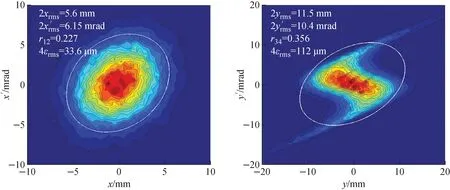
Fig.9 Reconstructed tomography in (x, x′) and in (y, y′) planes

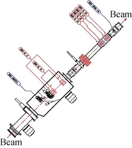
Fig.10 Drawing showing IMS section in which measurements we took for beam tomography were from quad IMS-Q17 to profile monitor IMS-RPM18; also emittance was directly measured with rig EMIT11

3 Measurements

Actual measurements were carried out in the ISAC mass separator (IMS) section[24]of LEBT in which there is an emittance rig equipped, allowing for direct measurement of the emittance. In order to minimize uncertainties which might exist for instance in the effective lengths of quadrupoles, the measurements for the tomography were taken in a very short section of the beam-line, that is, from the quadrupole IMS-Q17 to the profile monitor IMS-RPM18 (Fig.10, the distance between the EMIT11 and the RPM18 is about 2.806 m). This combination turns out to be a good choice because it creates a large enough rotation of phase spaces within the quad’s power supply output voltage limit. The beam used for the measurements was7Li+of 22.484 keV and ～5 enA, with negligible space charge effect. Prior to the data collection, some efforts were put to center the beam through the quad Q17, by adjusting the upstream steerers and then dithering Q17 until the beam centroid movement was barely noticeable at the monitor RPM18. This was a necessary step we had to take to ensure that there was no beam getting lost, due to feed-down effect, between Q17 and RPM18 over the entire range of the quad scan. Here our investigation focuses on the horizontal plane because the horizontal phase space has a peculiar shape and is of more interest than the vertical which is elliptical.Fig.11 show the horizontal beam profiles measured under various excitations of Q17 from 8 V to 1 708 V in a step of 100 V. They all appear to be clean. So only minor smoothing was used to process the data to clean up the isolated noises in the background. As expected, the square of 2rms sizes obtained from the profiles exhibit a good parabolic dependence on the voltage settings (Fig.12).

The beam tomography was first worked out at the entry of Q17, and then linearly transformed backwards passing through a section of 4 independent quads to the location of the emittance rig EMIT11 (Fig.10). The outcome is shown in Fig.13, along with the result directly measured with the emittance rig. They agree quite well in terms of the s-shape and the 2rms sizes, and the “mismatch factor” and the relative rotation between the two ellipses are no more than 15% and 20° respectively. This discrepancy possibly arises from inaccurate measures of the emittance rig’s orientation as well as the effective lengths of the quads in between as these quads have different effective lengths.

Moreover, we calculate the beam envelope to fit the measured beam sizes (2rms) of 36 values (18 inxand 18 iny) and therefore to find the sigma-matrix of beam at the location of EMIT11. This calculation, using statistical approach, serves as an independent double-check for the tomography analysis. There are only 6 initial parameters to be determined from the numerical fit, namelyαx,y,βx,yandεx,y, since the energy spread is nearly zero. So, the solution to be sought is over-determined. The fit achieves very good match for all the 36 values of beam size, and gives rise to an initial beam ofαy=0.547,βy=0.027 3 m, andεy=11.7 πmm·mrad in the horizontal plane. These give:

(11)

which appear to be exactly agreed with the tomography analysis results as displayed in the Fig.14 in white. The envelope calculation can’t tell the details about the shape of the 2D density distribution, though.

4 Conclusions

The maximum entropy algorithm has been validated at TRIUMF for the 2D transverse phase space tomography reconstruction, by using both the simulated models and the experimental measurements. This technique is applicable to the quadrupole scan and solenoid scan practices. In order to reduce distortions and errors in the reconstructed results, it’s essential to assure that the phase space rotation under the scans is larger than 90° and all the profiles are taken under exactly identical beam condition. This means that one must make sure that the scan range of the optical element is wide enough to cover a minimum beam size measured at the monitor, without changing anything to the beam condition during the scans (e.g. without any beam lost between the element scanned and the monitor recorded; and with no extra orbit steering added in the course). Moreover, the more scans one takes for the projections over the >90° rotation, the more accurate result one can achieve from the MENT reconstruction, but it’s not crucial to have an equal interval in the rotation angle of phase space. Also, it’s important that the measured beam profiles are properly processed and smoothed before input for the tomography reconstruction. Inconsistencies or artifacts among the profiles due to the noises and/or glitches have to be minimized. Under these conditions, convergence is usually achieved after 4-5 iterations. The tomography analysis can give more informative result than the statistical beam envelope calculation, particularly it can reveal the details of the 2D density distribution which are self-contained in the measured 1D projection profiles.

Fig.11 Horizontal beam profiles measured at monitor IMS-RPM18 under various voltage settings of quad IMS-Q17

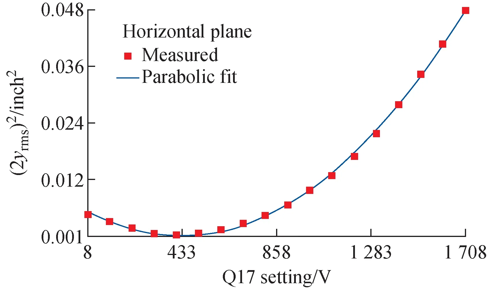
Fig.12 Square of beam size (2rms) measured at RPM18 vs. voltage setting of Q17

Fig.13 Tomography worked out at location of emittance scanner (left), and phase plot directly measured with emittance scanner (right)

We would like to thank the Beam Delivery Group and ISAC OPS for their support, coordination and help with the IMS measurements, also thank T. Planche for providing with the IMS optics model.

This work was funded by TRIUMF which receives federal funding via a contribution agreement with the National Research Council of Canada.