Jianing Dong(董佳宁), Yang Xiang(向阳), Hong Liu(刘洪), and Suyang Qin(秦苏洋)

School of Aeronautics and Astronautics,Shanghai Jiao Tong University,Shanghai 200240,China

Keywords: vortex ring,overpressure,back pressure,finite-time Lyapunov exponent(FTLE)

1. Introduction

Vortex rings widely exist in the wake of flying birds, insects,and swimming fish.[1]Jellyfish obtain suction thrust by generating vortex rings, which results in the lowest energy consumption ratio among all the animals.[2]Birds,bats and insects can generate closed vortex loops which increase the lift by 40%,with a maximum lift coefficient of 4.8.[3]Therefore,pulsed-jet propulsion is efficient because of the formation of vortex rings and their mutual interaction in the near wake.[4–6]

Vortex rings affect local pressure fields in moving animals’ wake, improving propulsive efficiency and contributing to high lift/thrust.[7]For example,jellyfish create counterrotating vortices along the outside of their bell margin. At the interface between these vortices,the accelerated fluid creates a high-velocity and low-pressure region on the forwardfacing surface of the bell margin.[8,9]This low pressure surrounding the bell generates a suction force that pulls the jellyfish forward. Simultaneously,the contracting bell propels the water backward, creating a high-pressure region that pushes the jellyfish forward. Krueger[10,11]proposed that the highpressure region augments thrust by reducing form drag. In a piston-cylinder apparatus, this high-pressure region is shown in Fig.1,which is the“back pressure region”for the rear vortex ring. Back pressure can enhance the vortex formation and bring a higher thrust to the nozzle. Back pressure affects vortex formation through overpressure, and overpressure causes additional impulseIP, which is associated with the entrainment process and composes the whole jet impulseITwith flux termIU[10,12]

Overpressure only exists in the acceleration phase in pistoncylinder apparatus,[13]accounting for at most of 40% of the total impulse in small formation timeL/D.[14–16]which means that the motion of a piston pushing a column of fluid of lengthLthrough a nozzle of diameterD. Back pressure affects overpressure, which directs to the formation enhancement of vortex rings. Detailed studies should be conducted to discover the potential influence.

Previous studies on the interaction of vortex rings mainly focus on kinematic phenomena. Leapfrogging and merger are experimentally observed in dual vortices interaction.[17]Fu[18]found that for two continuous generated vortex rings, the latter formed one gains at most of 80%augmentation in impulse compared with an isolated vortex ring with the same formation number. In multiple vortex rings,Krueger[11]generated a string of identical vortex rings intermittently and found that the largest relative force would occur at small formation time and large interval.Qin[19]proposed two interaction modes:formation enhancement mode with open flux window and formation restraint mode with closed flux window. The flux windows allow fluid to transport and entrain,generating additional circulation in vortex formation by increasing overpressure.However,the current studies have not revealed how overpressure is affected by the interaction of vortex rings, and the effect of back pressure on overpressure is still unknown. Therefore,the pressure evolution in the interaction of vortex rings is important and needs to be detailed.

Fig. 1. Schematics of back pressure and overpressure region in dual interacting vortex rings.

In conclusion, the research in this paper starts from the scientific problem of the mechanism of animals’ efficient propulsion by vortex ring. Based on the observation of jellyfish,the extra thrust is brought from the interaction of vortex rings by changing the flow field’s pressure. However, there is little research on the interaction of vortex rings from the perspective of pressure. Consequently,this paper explores the effect of back pressure on overpressure in dual interacting vortex rings and reveals their influence on the formation of vortex rings. The rest of this paper is arranged as follows. The experimental setup and the calculation methods of flow field parameters are introduced in Section 2. Section 3 presents the evolution of back pressure under different formation times and interval times. Section 4 reveals the relationship between back pressure and overpressure and proposes a critical distance for vortex formation. Finally,the main conclusions from this study are summarized in Section 5.

2. Method

2.1. Experimental setup

The layout schematic of the apparatus in this experiment is shown in Fig. 2. The basic system consists of two pistoncylinder apparatus: the vertical driving section and the horizontal jet section. These two sections are immersed in a water tank(2.8 m in length×1 m in width×1.2 m in depth). Due to the incompressibility of water, the floating piston in the horizontal cylinder follows the movement of the driving piston jointly driven by the stepper motor. The exit of the cylindrical nozzle has an inner diameter ofD=50 mm,and the outer wall of the nozzle near the exit is sharpened to form a wedge of 17◦. In addition, the tank was sufficiently large to avoid wall effects.[20]

The flow field is observed by DPIV. The flow is seeded with hollow, silver-coated, neutrally buoyant glass spheres with diameters within the range of 30–50 µm. The particles are illuminated with a 10W Nd: YAG laser whose beam is formed into a 2-mm-thick sheet by using a cylindrical lens. A CCD camera with a resolution of 2320×1200 pixels and a 50 Hz frame rate records the motion of particles mounted in front parallel to the laser sheet. Particle movement is analyzed to determine the two-dimensional velocity vector of flows,and a window shifting algorithm is used to cross-correlate the images with a 64×64 pixels correlation window size and a 16×16 pixels moving average step size,which results in one velocity grid point with 8 pixels. Therefore, a velocity field of 290×158 grids with a spatial resolution of 0.14×0.13 cm is obtained. By satisfying the constraints(interval time,particle size,and particle concentration)of the DPIV measurement and after alignment, the velocity measurement and vorticity calculation uncertainties are 1%and 3%,respectively.[19]

Fig. 2. Schematic of a piston-cylinder apparatus with digital particle image velocity(DPIV).

Arduino Board Mega 2560 is used to control the stepper motor, which is a development microcontroller board for writing velocity program. Two vortex rings with the same formation time are successively produced with interval time ranging from 0 to 3 s. The velocity type is sinusoidal with a maximum of 0.05 m/s, as shown in Fig. 3. The purpose of this velocity profile is to reduce or even eliminate the formation of a stopping vortex around the exit of the nozzle at the end of each stroke. For a little dilation of the flexible hose and the friction from the jet piston, the actual velocity in nozzle exit has a slight deviation from the sinusoidal type.The error of stroke length is within 1%, which satisfies the requirements for stroke accuracy. The Reynolds number for these non-impulsively started velocity programs is defined asRe=UmaxD/ν, where the nozzle diameterDis 0.05 m, and fluid viscosityvis 10−6m2/s. As theUmaxin our experiment is 0.05 m/s,the corresponding Reynolds numberRein all the cases is 2500.

Fig. 3. Sinusoidal velocity program. ∆t is the time interval ranging from 0.5 s to 3 s.

The naming method is illustrated as follows. In the case named asn–m–k, the first numbernis the formation timeL/D=n, the second onemcorresponds to the number ofmstrokes in a row, and the last onekis the interval time∆t=k×10−2s between two strokes,which is marked in Table 1.

Table 1. Summary of experimental parameters. The cases are named by L/D-strokes numbers-time intervals. L/D is the formation time,∆t is the time interval between two successive strokes.

2.2. Finite-time Lyapunov exponent field

As the Lagrangian skeleton of flow,Lagrangian coherent structures (LCSs) provide a geometrical view of flow structures and characterize fluid transport and deformation over a certain period.[21,22]Although there are some inconsistencies,the ridges of the FTLE are heuristic indicators of hyperbolic Lagrangian coherent structures.[19,23,24]This paper applies the FTLE ridges to analyze the fluid transport. Applyingφt+T t:x(t)→x(t+T) to denote the flow map of a material point located atx(t)at timetto its position at the timet+T,the deformation gradient is

Then,FTLE is computed by

whereλmax[∆(x,t0,T)] is the maximum eigenvalue of∆(x,t0,T).|T| is used because FTLE can be computed forT>0 andT<0. Regions of maximum fluid-particle separation (forT>0) or maximum fluid particle attraction (forT<0)produce local maximizing curves known as“ridges”in the FTLE.The ridges in forward-time FTLE(T>0)reveal repelling hyperbolic LCSs(r-LCSs)and the ridges in backwardtime FTLE (T< 0) reveal attracting hyperbolic LCSs (a-LCSs).[19]The integration time|T|is chosen according to the particular flow being analyzed.The maximum integration time for each case in our experiments is 2.00 s,which is sufficient to get the clear ridges of FTLE fields.

What’s more, the clarity of FTLE ridges depends on the number of calculating frames of the forward-time FTLE and backward-time FTLE. The higher the number of calculating frames,the clearer the FTLE ridges,and the longer the calculation takes. However, because the FTLE is calculated from DPIV data, there is an upper limit on the clarity of FTLE ridges due to the original grids(290×158). After testing with different calculating frames, 100 calculating frames are selected in this experiment. When it is less than 100,the boundaries of vortex rings are not clear enough; when it is greater than 100,the clarity is not much improved than those of 100.Therefore,the flow fields in the following content are already close to their highest resolution and sufficient for further analysis.

2.3. Pressure field calculation

The method to calculate the pressure fields is based on the algorithm proposed by Dabiri.[25,26]The pressure gradient is estimated from a time series of velocity fields for unsteady calculations or a single velocity field for quasi-steady calculations. The approaches for pressure field estimation is based on direct integration of the pressure gradient term in the Navier–Stokes equation,e.g.,for incompressible flow

In order to reduce the effect of measurement errors that accumulate along individual integration paths,the integration result is chosen as the median polling of 8 integration paths.Furthermore,the primary source of measurement error in this type of unsteady estimate of the material accelerationDu/Dtarises from temporal noise in the measured velocity components at each node in the velocity field,where

wheretis the temporal sequence of velocity fields to be analyzed,uτis a velocity vector corresponding to velocity fieldtin the sequence,u∗τis the spline-approximated value of the same velocity vector for the same velocity field,φis a weight between the first and rear terms and is validated to be chosen as 0.05 in both steady and unsteady situation.[25]Finally,the viscous term on the right-hand side of Eq.(5)is computed using finite centered differences between adjacent nodes in the velocity field,and then we could integrate the pressure in Eq.(6).The boundary pressure, which the integration starts, is set as zero.

As for the resolution of the pressure field,same as FTLE,it is calculated from the velocity field with the same resolution as 290×158 grids. In addition, there is no need to increase the resolution through grid difference because it has little influence on the calculation of pressure field and costs much longer. What’s more, the velocity would be smoothed by spline-approximated in the MATLAB program,which has a similar effect as the velocity difference. Consequently,the obtained pressure fields are clear enough for the following qualitative analysis.

2.4. The calculation of back pressure circulation

After obtaining the pressure of the whole flow field, we choose the “back pressure characteristic point” to calculate back pressure circulation, which is at the intersection of the front boundary and the centerline of the vortex ring bubble,moving with vortex ring during the formation process. As the vortex ring is regarded as an ellipsoid,the position of the intersection is determined by the sum of the moving distance of the vortex ring and its short semiaxis. The vortex rings’kinematic parameters are as follows:[27]

We get the moving distance of vortex rings by integratingV0with time, and multiply aspect ratioγ=0.6 with the long semiaxisRbto get the short semiaxis of the vortex,then add these two together to obtain the position of intersection.The position of“back pressure characteristic point”is shown in Fig. 1, the solid green circle. The parameters in Eqs. (10)and(11)are detailed in the study of Sullivan.[27]

The overpressure circulationΓpis calculated as

wherepbclis the back pressure.Γbrepresents the total influence of back pressure on vortex formation,and can be compared in the same dimension withΓp.

3. The evolution of back pressure

In the previous studies,Krueger[10]and Qin[19]found that interval space between vortices significantly influences their interaction. The interval space during the formation phase is determined by two factors: the interval time and translation velocity. The translation velocity is related to vortex ring size,which is determined by formation timeL/D. To analyze the influence of interval space on back pressure,we use the DPIV data obtained from experiments to calculate the flow fields and pressure fields by the methods mentioned in Subsection 2.2 and Subsection 2.3. The analysis is as follows.

Firstly,we investigate the flow and pressure fields of different interval times with the same formation time. The cases ofL/D=2 are chosen as examples. The fields of the midpoint time are selected and shown in Fig.4. Figures 4(a)–4(d)are the flow fields,presenting the cases 2-2-05,2-2-10,2-2-20 and 2-2-30,respectively. In case of 2-2-05(a),a flux window between the dual vortex rings is composed of connected LCS contour between the rear and the front. With ∆tincreasing,the interval space extends larger, and the flux window gradually disappears(b)–(d). Figures 4(e)–4(h)are the corresponding pressure fields. The back pressure reaches a maximum in case 2-2-05(e)and begins to decline in case 2-2-10(f),where the flux window gradually disappears. Whereas, as shown in cases 2-2-20(g)and 2-2-30(h),the back pressure rises again after the flux window disappears with a strong barrier formed back the front vortex ring.

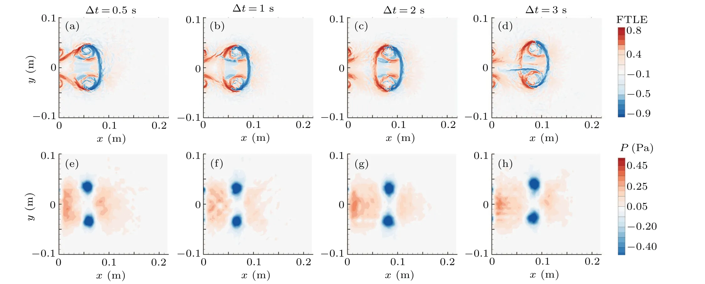
Fig.4. The midpoint of the rear vortex formation in cases of L/D=2 with four different time intervals. (a)–(d)Flow fields. (e)–(h)Pressure fields.

Secondly, we investigate the flow and pressure fields of different formation times with the same interval time. The cases ofL/D=2 andL/D=4 with ∆t=1 s are taken as examples. The beginning, end, and the midpoint of the rear vortex ring’s generation are shown in Fig. 5. Even within the same time interval, a vortex ring with a small formation time moves slower (a)–(c), in which a flux window occurs at the midpoint of formation. On the contrary,the vortex moves faster with a large formation time(d)–(f),the front vortex ring has grown completely at the beginning of the rear vortex formation. Therefore,a distinct closed FTLE ridge forms and no flux window occurs.

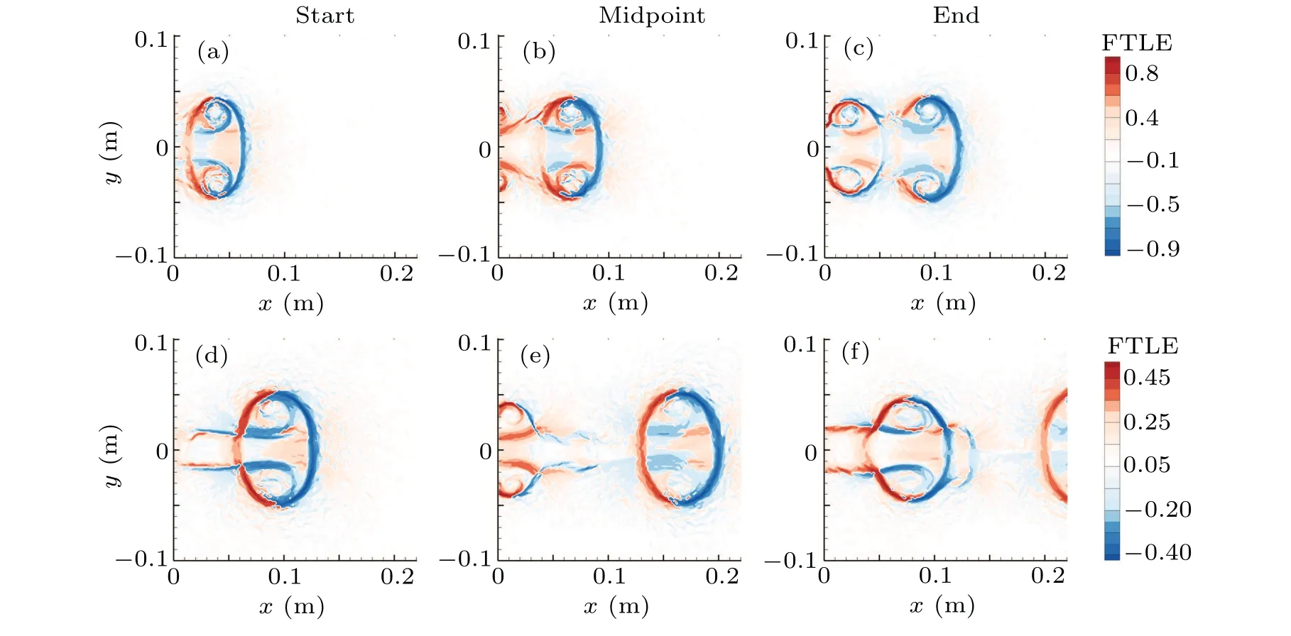
Fig.5. The flow fields of start,end,and the midpoint of the rear vortex ring’s formation with time interval is 1 s. (a)–(c)L/D=2. (d)–(f)L/D=4.

The corresponding pressure field is shown in Fig. 6, as shown in Figs.6(b)and 5(b).The maximum back pressure occurs when the flow window exists, similar to Figs. 4(a) and 4(e). It is indicated that the flux window can bring higher back pressure. Figures 6(d)–6(f) and 5(d)–5(f) reveal that a detached high-pressure region forms at the beginning of the rear vortex ring with a large formation time and then begins to polymerize when the rear vortex ring propagating downstream faster,which makes the back pressure rises again.

In order to explore the joint effect of interval time and formation time on back pressure in detail, the evolution of back pressure over time in all the experimental cases in Fig.7. For small formation time(L/D ≤2),under four different time intervals,the evolution of back pressure is similar:it reaches the peak at the beginning of formation and then decreases down to negative in the end. The high back pressure is caused by the flux window,which disappears as the interval distance increases.

Fig.6. The pressure fields of start,end,and the midpoint of the rear vortex ring’s formation with time interval is 1 s. (a)–(c)L/D=2. (d)–(f)L/D=4.

Fig.7. Back pressure evolution over the whole period of the rear vortex formation in all experimental cases.

Moreover,due to the influence of the leading vortex,the back pressure goes from positive to negative. The situation is the opposite of large formation time: in the cases ofL/D=4,the back pressure gradually increases and reaches the peak near the end. It is caused by the change of the high-pressure region between the two vortices: at first, the low back pressure is caused by the detached high-pressure region,as the rear vortex propagates downstream,the interval distance shortens,which polymerizes the separated high-pressure region,leading to back pressure rises. As for the cases ofL/D=3,the back pressure develops relatively stable. In conclusion, with the increase ofL/D, back pressure in vortex formation changes from negative correlation to positive correlation with formation time,which indicates the importance of formation time to back pressure.

4. The effect of back pressure on overpressure and formation of vortex rings

4.1. Circulation of the flow field

The interaction between vortex rings influences vortex ring formation, which is manifested as the circulation when the vortex ring finishes formation. For the circulation calculation, the velocity obtained by DPIV is used to calculate the vorticity in Fortran, which is integrated over the upper half field and the lower half field to get the circulation of the upper and lower vortices. Finally, their average is taken as the final circulation of the vortex ring. We calculate the circulation of vortex rings in all cases and those ofL/D=2 are shown in Fig.8 as examples.

Fig.8. Circulation increase of L/D=2 as a function of real-time.

We first calculate the circulation of an isolated vortex ring,marked as the solid black square in Fig.8,then subtract it from total circulation to get the circulation of the rear vortex ring. Referring to the impulse in Eq.(1),the vortex ring’s circulation also originates from jet flux and overpressure[14]

The circulation contributed by jet fluxΓUis estimated by slug model

The jet fluxΓUis constant in the same formation time. Thus,the circulation difference can only be caused by the overpressureΓp. Therefore, we subtractΓUfromΓTto getΓp, which can both manifest the overall circulation and overpressure’s evolution.

4.2. Synchronization of overpressure and back pressure

Referring to Eq.(13),the back pressure circulation is calculated to represent the total influence of back pressure on vortex formation, and can be compared in the same dimension withΓp. The relationship ofΓbandΓpis shown in Fig.9. The superscript∗ofΓbandΓpis referred to as the dimensionless byUmaxD. There is a strong linear relationship betweenΓ∗bandΓ∗p: a linear fitting formula isΓ∗p=1.56Γ∗b+0.16, the correlation coefficient is 0.8,r-square(adj.) is 0.62. It is indicated that back pressure has a positive effect on overpressure.Even in the absence of direct measurement of overpressure,based on the synchronous ofΓbandΓp,we can indirectly find that higher back pressure can lead to higher overpressure in the early stage of vortex formation. As a result,a larger vortex ring with higher circulation formed. Therefore,we can predict the formation of vortex ring byΓb. WhenΓbreaches its peak,the vortex formation can be most stimulated. As mentioned in chapter III,in smallL/D,the initial interval distance is narrow,the high back pressure comes from the flux window; in largeL/D, the initial interval distance is wide, the high back pressure comes from the regrouped high-pressure region. Thus,we can use the initial interval distance to distinguish between the two forms of high back pressure formations,and there may exist a“critical distance”.When the rear vortex is generated at this“critical distance”from the front,Γbreaches its maximum.

Fig. 9. The evolution of overpressure circulation with back pressure circulation. The rectangle, circle, triangle, and diamond represent the cases of L/D=1,2,3,and 4,respectively.

4.3. Critical distance for the formation

As the initial interval distance and the back pressure circulation are positivel related to the formation timeT∗,in order to eliminate the influence ofT∗on back pressure,we normalizeΓ∗bbyT∗to manifest the unit back pressure circulation.Besides,we measured the initial interval distanced,which is the distance between the two vortex cores when the rear vortex begins to grow. In order to eliminate the influence ofT∗ond,a dimensionless distance is defined as

whereDis the nozzle diameter.

Fig.10. (a)The evolution of unit back pressure circulation with dimensionless interval distance. The black diamonds,circles and squares are experimental cases and form a trend band. (b) The pressure fields at the beginning and end of the rear vortex formation. I,II,and III are the regions corresponding to(a).

The evolution ofΓ∗b/T∗withd∗is shown in Fig. 10(a).With the increase ofd∗,Γ∗b/T∗increases first and then decreases, shown as the blue band. To explain the formation of this trend band,we analyzed the pressure field of all cases and found three distinct pressure fields. Therefore,all cases are divided into three regions:part I,part II and part III.Each case in each region has similar back pressure evolution and is labeled as diamond, circle and square, respectively. Furthermore, the two dividing lines that distinguish the three parts ared∗=0.32 andd∗=0.42,between which a criticald∗exists corresponding to the maximum ofΓ∗b/T∗. The criticald∗is labeled asd∗crwith a range of 0.32–0.42.

In order to show the differences of back pressure evolution among the three regions, we selected the representative case in each region: case 1-2-05 represents part I,case 4-2-05 represents part II,and case 3-2-30 represents part III.Theird∗are 0.2, 0.4 and 0.6 respectively. Their pressure fields at the beginning and end of the rear vortex formation are shown in Fig. 10(b). An over-interaction mode occurs in part I, where the interval distance is too narrow for back pressure to grow and the leading vortex’s negative pressure dominates the interval space; a full-interaction mode occurs in part II, where the interval distance is the most suitable, and the back pressure reaches its maximum; an under-interaction mode occurs in part III, where the interval distance is too broader, and the back pressure is low due to the detached high-pressure region.

5. Conclusion

Experiments are conducted to examine the vortex formation and pressure evolution in dual interacting vortex rings.Two vortex rings, which have the same formation timeL/D,are successively generated in a piston-cylinder apparatus. By controlling the formation time and the interval time, we explore the effect of back pressure on the formation of the rear vortex ring. We find that the back pressure is high in the flux window region whenL/Dis small. In largeL/D, high back pressure is caused by the regrouped high-pressure region.Moreover, the back pressure changes from a negative correlation to a positive correlation with formation time asL/Dincreases. Furthermore, we find a strong linear relationship between the back pressure and overpressure. Therefore, the formation of vortex ring can benefit most from the interaction when the back pressure is the highest. In order to find a unified highest back pressure criterion under allL/D,we get the evolution of unit back pressure circulationΓ∗b/T∗with dimensionless interval distanced∗. As a result, with the increase ofd∗,Γ∗b/T∗first increases and then decreases, so there is a criticald∗crcorresponding to the maximum unit back pressure circulation.At this point,a full-interaction mode appears,in which the interaction has the best promoting effect on the formation of vortex ring. Whend∗d∗cr, the formation of vortex ring is weakly affected by the interaction, so there is an under-interaction mode occurs between the two vortices.

Acknowledgements

Project supported by the National Natural Science Foundation of China (Grant Nos. 12102259 and 91941301)and China Postdoctoral Science Foundation(Grant No.2018M642007).