Shenming FU, Jingping ZHANG, Yali LUO, Wenying YANG, and Jianhua SUN

1International Center for Climate and Environment Sciences, Institute of Atmospheric Physics,Chinese Academy of Sciences, Beijing 100029, China

2University of Chinese Academy of Sciences, Beijing 100049, China

3Laboratory of Cloud–Precipitation Physics and Severe Storms, Institute of Atmospheric Physics,Chinese Academy of Sciences, Beijing 100029, China

4State Key Laboratory of Severe Weather, Chinese Academy of Meteorological Sciences, Beijing 100081, China

5Collaborative Innovation Center on Forecast and Evaluation of Meteorological Disasters,Nanjing University of Information Science and Technology, Nanjing 210044, China

ABSTRACT Predicting warm-sector torrential rainfall over South China, which is famous for its destructive power, is one of the most challenging issues of the current numerical forecast field. Insufficient understanding of the key mechanisms underlying this type of event is the root cause. Since understanding the energetics is crucial to understanding the evolutions of various types of weather systems, a general methodology for investigating energetics of torrential rainfall is provided in this study. By applying this methodology to a persistent torrential rainfall event which had concurrent frontal and warmsector precipitation, the first physical image on the energetics of the warm-sector torrential rainfall is established. This clarifies the energy sources for producing the warm-sector rainfall during this event. For the first time, fundamental similarities and differences between the warm-sector and frontal torrential rainfall are shown in terms of energetics. It is found that these two types of rainfall mainly differed from each other in the lower-tropospheric dynamical features, and their key differences lay in energy sources. Scale interactions (mainly through downscale energy cascade and transport)were a dominant factor for the warm-sector torrential rainfall during this event, whereas, for the frontal torrential rainfall,they were only of secondary importance. Three typical signals in the background environment are found to have supplied energy to the warm-sector torrential rainfall, with the quasi-biweekly oscillation having contributed the most.

Key words:torrential rainfall,warm-sector rainfall,frontal rainfall,South China,scale interactions,baroclinic energy conversion

1.Introduction

The rainy season in China begins earliest in South China (18°–26°N, 105°–120°E) (Tao, 1980). Torrential rainfall occurs frequently during South China’s rainy season and contributes ～50% to the total precipitation during this period (Sun et al., 2019). Warm-sector torrential rainfall is a special type of torrential rainfall that occurs over South China (Huang, 1986; Liu et al., 2019; Fu et al., 2020). It is defined as the torrential rainfall which appears (1) in a warm sector that is approximately 200−300 km away from a surface front; or (2) in the convergent area between southeasterly and southwesterly winds; or (3) in a region dominated by southwesterly wind but without wind shear. These three situations are not directly controlled by tropical systems (e.g., typhoons). Warm-sector torrential rainfall often occurs suddenly, which results in strong and concentrated precipitation(Lin et al., 2006; Chen et al., 2018b; Luo et al., 2020). Due to its lower predictability and strong intensity, warm-sector torrential rainfall often results in severe economic losses and heavy casualties (Luo et al., 2017; China Meteorological Administration, 2018; Li et al., 2020).

For decades, persistent efforts have been made to further the understanding of warm-sector torrential rainfall (Kuo and Chen, 1990; Zhou, 2000; Ding et al., 2006; Zhang et al.,2011; Jou et al., 2011; Luo et al., 2017). It is found that warm-sector torrential rainfall accounts for more than 15%of the torrential rainfall in South China (Liu et al., 2019).This type of rainfall mainly occurs during the pre-rainy season(April to June), and it exhibits a larger occurrence number over the eastern coastal regions than the inland regions(Huang, 1986; Chen et al., 2012). Although not directly affected by a front, warm-sector torrential rainfall could occur with frontal precipitation concurrently, but its intensity is stronger than that of frontal precipitation (Huang, 1986;Lin et al., 2006; Li et al., 2020). Previous studies (He et al.,2016; Liu et al., 2016; Miao et al., 2018) have proposed that favorable conditions for warm-sector torrential rainfall mainly include four situations: (1) a convergent flow or a warm and moist wind shear behind a transformed cold high pressure system, (2) a strong southwestern monsoon surge or southwestern low-level jet, (3) an upper-level trough and a subtropical low-level jet, and (4) a mesoscale vortex. Two trigger mechanisms are found to be dominant. One is mainly due to the wave or lifting effect produced by the inhomogeneous underlying surface of South China (Xu et al.,2012; Chen et al., 2015, 2016), and the other is mainly due to instability (Ding and Shen, 1998), density currents (Houston, 2017), and gravity waves (Liu et al., 2012; Xu et al.,2013). Although previous studies have advanced the understanding of warm-sector torrential rainfall, thus far, predicting this type of event remains one of the most challenging issues in the numerical forecast field (Wu et al., 2018,2020b). For example, all current operational numerical weather prediction models failed to forecast the severe warm-sector torrential rainfall over Guangzhou on 7 May 2017, which resulted in economic losses of approximately 180 000 000 RMB and casualties of over 20 000 (Tian et al.,2018; Wu et al., 2018). One of the most important reasons that warm-sector torrential rainfall is challenging to forecast is that there is still a lack of sufficient understanding about its key mechanisms (Sun et al., 2019).

Understanding the energetics is crucial to understanding the evolutions of different types of weather systems (Lorenz,1955; Plumb, 1983; Kucharski and Thorpe, 2000;Murakami, 2011; Wang et al., 2016; Fu et al., 2018). However, thus far, no studies have provided a physical image of the energetics of warm-sector torrential rainfall, let alone detailed the main differences between warm-sector and frontal torrential rainfall in terms of energetics. Therefore,the primary purpose of this study is to fill these two research gaps. The remainder of this article is organized as follows: the data and method are described in section 2; an overview of the selected event is provided in section 3; the physical image of energetics is provided in section 4; and a conclusion and discussion are given in section 5.

2.Data and method

2.1.Dataset

The hourly, 0.25o× 0.25oERA5 reanalysis data from the European Centre for Medium-Range Weather Forecasts(Hersbach et al., 2020), available on 37 vertical levels, is used in this study to calculate energy budgets and to conduct empirical orthogonal function (EOF) (Weare and Newell,1977) analysis (which is used to determine the dominant mode of eddy flow during this event). A 30-min, 8-km precipitation dataset, produced by using the US Climate Prediction Center morphing technique (CMORPH), is employed to investigate precipitation variation and to conduct the wavelet analysis (Erlebacher et al., 1996). The CMORPH data is verified via comparison with gauge observations to provide a credible estimate of precipitation over South China (Shen et al.,2010).

2.2. Method

This study uses two types of energies: available potential energy (APE) and kinetic energy (KE), which are effective measurements for the thermodynamical and dynamical conditions of the real atmosphere, respectively. Since torrential rainfall is directly caused by eddy flow, which is embedded in a favorable background environment (Markowski and Richardson, 2010; Fu et al., 2015, 2016), we utilize an energy analysis method that can reflect the variations of both eddy flow and its background environment (Murakami, 2011). The budget equations are as follows:

where the overbar represents an N-day temporal average. A sample basic variable S (e.g., zonal wind u, meridional wind v, vertical velocity ω, specific volume α, temperature T, potential temperature θ, geopotential Φ) can be decomposed as, wheredenotes the background environment (contains signals with periods >N days) and S’ represents eddy flow (contains signals with periods ≤N days). AMand KMdenote APE and KE of the background environment,respectively; ATand KTrepresent APE and KE of eddy flow,respectively. AIand KIare APE and KE of the interaction flow, respectively, which are developed to link eddy flow to its background environment (Murakami, 2011; Fu et al.,2016, 2018). The physical meaning of each term is shown in Table 1.

Scale interactions between eddy flow and its background environment can occur directly through energy cascades.The energy cascade terms of the APE are C(AM,AI) and, which have a relation:F(AI) , where F(AI) represents transport of AIby eddy flow.When C (AM,AI)>0 and, AM→AI→AT, i.e., a downscale APE cascade occurs (Table 1). If C(AM,AI)<0 and, AT→AI→AM, i.e., an upscale APE cascade occurs. Otherwise, no energy cascade occurs.The energy cascade terms of KE are C(KM,KI)=and, where div(·)is the divergence operator; u is the three-dimensional wind vector (u =u+u′); φ is latitude; grad ( ) is the gradient operator; and a is the Earth’s radius. Their relation is, where F(KI) represents transport of KIvia eddy flow (Table 1). A downscale KE casca(de (K)M→KI→KT) occurs when C(KM,KI)>0 and<0, and an upscale KE cascade (KT→KI→KM)appears when C (KM,KI)<0 an(d. Otherwise,no KE cascade occurs. Termcan be decomposed into two parts. The first part (FP) is, which denotes three-dimensional transport of KTby the background environment. It can be regarded as a type of scale interaction between eddy flow and its background environment via transport. The second part (SP) iswhich represents three-dimensional transport of KTand Φ’by eddy flow. Detailed physical significances, expressions,and spheres of application for Eqs. (1)–(4) are provided by Murakami (2011) and Fu et al. (2016).

Table 1. Terminology used in this study, where symbols “→” and “←” denote the directions of energy conversion.

3.Overview of the selected torrential rainfall event

The selected event occurred in the pre-summer rainy seasonaThis event was chosen because (1) its intensity, spatial distribution, and background environment were similar to the typical situations summarized in a 34-yr statistical study (Liu et al., 2016); (2) it had remarkable concurrent rainbelts (Fig. 1a) over inland (frontal precipitation) and coastal regions (warm-sector precipitation), that are a prominent feature for East Asian monsoon rainfall over South China (Du and Chen, 2019a; Li et al., 2020); and (3) it caused extensive flooding and severe urban waterlogging over South China, resulting in huge economic losses (Sun et al., 2019). These features ensure the representativeness of the selected event., and its relatively heavy precipitation mainly appeared during a 72-h period (from 1200 UTC 15 to 1200 UTC 18 June 2017). Therefore, a 72-h time window is used to calculate the eddy flow (section 2.2). As Fig. 1a shows,strong-KTregions corresponded to the accumulated preci-pitation well, implying the key role of eddy flow in producing the torrential rainfall. The first EOF mode of the eddy flow(variance contribution was ～40%) indicates that, the eddy flow featured a northeast–southwest oriented shear line (Fig.1b), which corresponds to the front shown in Fig. 2. To focus on the torrential-rainfall-related eddy flow, a key region (KR; green boxes in Fig. 1a) is chosen to cover the main body of the strong-KTregions. According to the shear line’s location, the KR is divided into northern and southern sections (Fig. 1c), which are of equal size.

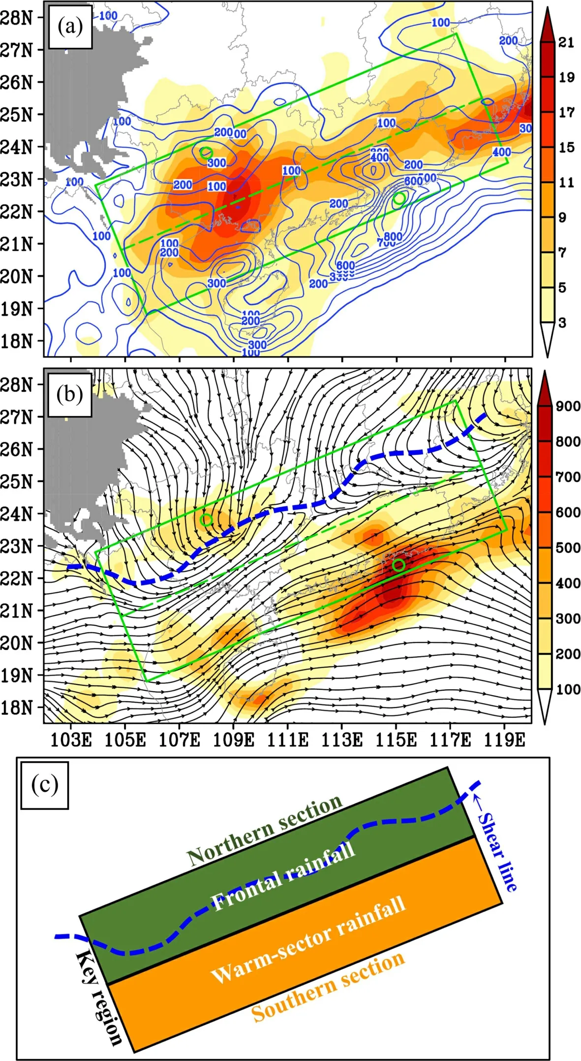
Fig. 1. Panel (a) shows the 72-h (from 1200 UTC 15 to 1200 UTC 18 June 2017) accumulated precipitation (mm; the thickest contour denotes 50 mm)and the 72-h temporal mean of the lower-level KT (J kg–1; shading). Panel (b)illustrates the 72-h accumulated precipitation (mm; shading) and the dominant mode of the lower-level eddy flow, where the stream field is composited by the respective first EOF modes of the zonal and meridional winds at the lower level. Here, all lower-level features are represented by a vertical mean from 950 hPa to 850 hPa. The green tilted box marks the key region, with a dashed green line dividing it into the northern and southern sections. Grey shading shows the terrain above 1500 m, small green circles mark the focused precipitation centers of frontal and warm-sector rainfall,respectively, and the thick blue dashed line represents the lower-level shear line. Panel (c) is a schematic illustration of the configuration of the two types of rainfall.

The northern section was governed by a shear line/front(Fig. 1b), with the heaviest precipitation (>400 mm) appearing around (23.5°N, 108°E), over the inland regions. As the cross section through this rainfall center (Fig. 2a) shows,there was a notable frontal structure that was characterized by a large horizontal temperature gradient, strong convergence below 700 hPa, and strong ascending motions in the middle and lower troposphere. The heavy precipitation was induced mainly by the front and thus is classified as frontal rainfall (Fig. 1c). In this section, the lower-level strong KT(Fig. 1a) was mainly associated with the shear line(Fig. 1b).

Fig. 2. Vertical cross sections along two typical longitudes (108°E and 115°E) where the maximum 3-h rainfall centers appeared. The shadings represent wind divergence (10–5 s–1), the red lines are temperature(°C), the vectors denote the wind vectors of meridional (m s–1) and vertical motion (cm s–1). The purple open bars mark the location of the maximum 3-h rainfall center with its amount being labeled in purple numbers.The two blackish green dashed lines outline the frontal zone, while the purple dashed ellipses with arrow heads show the direct thermal circulation. The grey shading in (a) shows the terrain.

The southern section of the KR was mainly located in the warm sector of the front (Fig. 2b), and the heaviest precipitation (>900 mm) occurred around (22.5°N, 115°E), near the coast. As the cross section through this rainfall center(Fig. 2b) shows, heavy precipitation was mainly located in the warm sector that was ～200 km away from the surface front. Therefore, this area of rainfall should be classified as warm-sector precipitation (Fig. 1c). In this section, the lower-level strong KTwas mainly associated with the intense southwesterly wind (not shown).

There was a favorable background environment during the selected torrential rainfall event. In the upper troposphere, the KR was located within the eastern section of the South Asia high, where the wind field was anticyclonic with strong divergence (Fig. 3a). This was conducive to maintaining ascending motion at the lower levels. In the middle troposphere, a shortwave trough was situated aloft with respect to the KR (Fig. 3b). Around the trough, there were westerly winds and a temperature field which decreased towards the southeast, both of which resulted in warm advection. The warm advection aided in maintaining/enhancing lower-level upward motion through quasigeostrophic forcing (Holton,2004). In the lower troposphere, a notable transversal trough controlled the northern section (Fig. 3c), and a strong southwest monsoonal wind dominated the southern section.The monsoonal wind caused a net import of moisture and energy into the KR, which was favorable for precipitation.

Fig. 3. Panel (a) shows the 72-h time-averaged (from 1200 UTC 15 to 1200 UTC 18 June 2017) divergence (shading,units: 10–5 s–1), geopotential height (black solid lines, units: gpm), and wind field (a full wind barb is 10 m s–1) at 200 hPa. Panel (b) illustrates the 72-h time-averaged geopotential height (black solid lines, units: gpm),temperature advection (shading; 10–5 K s–1), temperature (red lines, units: oC), and wind exceeding 5 m s–1 (a full wind barb is 10 m s–1) at 500 hPa. Panel (c) depicts the 72-h time mean of the vertically averaged (from 950 hPa to 850 hPa) geopotential height (black contours, units: gpm) and wind exceeding 2 m s–1 (a full bar is 4 m s–1). In panels (a and b), the thick grey curved lines outline the terrain above 3000 m, the tilted green box shows the key region, and the brown dashed line marks the trough line. In panel (c), the green tilted box marks the key region, with a dashed green line dividing it into the northern and southern sections. Grey shading shows the terrain above 1500 m,and the brown dashed line marks the trough line.

4.Physical image of energetics

4.1. Separations of the original meteorological field

A Morlet wavelet-based analysis (Erlebacher et al.,1996) is applied to the 30-min, key-region averaged CMORPH precipitation (using data from 1 April to 1 October). The result indicates that the torrential-rain-producing eddy flow was mainly governed by a quasi-daily signal(Figs. 4a and b). This is consistent with the findings of Jiang et al. (2017), Chen et al. (2017), Chen et al. (2018a), and Wu et al. (2020a), as they all confirmed the notable diurnal variations of heavy precipitation over South China. As Figs.4a and b show, the background environment of this event was jointly dominated by a quasi-weekly oscillation (QWO;over 95% confidence level), a quasi-biweekly oscillation(QBO; over 90% confidence), an intraseasonal oscillation(ISO; over 90% confidence level), and oscillations with longer periods (these signals cannot be identified by using a half-year dataset). A schematic illustration of the wavelet analysis is shown in Fig. 4c.

Fig. 4. Wavelet analysis of the target region-averaged precipitation by using Morlet wavelet-based analysis. Panel (a)shows the wavelet power spectrum (shading), where grey dots mark the regions exceeding the 95% confidence level,and the two black dashed lines show the 72-h time window of this event. The thick black solid curved line indicates the cone influence outside of which the edge effect become important. Panel (b) illustrates the 72-h mean wavelet power spectrum during the event (thick red line), where purple and green dashed lines outline the notable signals in the background environment, and the thick grey solid line shows the position of the 3-day running mean (which separates the original time series into the eddy flow and its background environment). Panel (c) is a schematic illustration of the wavelet analysis results, where blue bold characters show the typical signals. BE = Background environment; QDS = Quasi-daily signal; QWO = Quasi-weekly oscillation; QBO = Quasi-biweekly oscillation; ISO =Intraseasonal oscillation.

The northern and southern sections of the KR experienced completely different torrential rainfall; one experienced frontal precipitation, and the other experienced warmsector precipitation. Nevertheless, in terms of AMand KM,the northern and southern sections of the KR exhibited similar features (e.g., vertical distribution, peaks) to those of the whole KR (Figs. 5a and b). This means that the frontal and warm-sector precipitation shared a similar background environment. For the torrential-rainfall-related eddy flow, in the middle and upper troposphere, ATand KTwithin the northern and southern sections exhibited similar features to those of the whole KR (Figs. 5c and d). However, in the lower troposphere, the KTvalues within the two sections notably differed from each other (Fig. 5d). This means that the essential differences between frontal and warm-sector rainfall mainly lay in the dynamical features in the lower troposphere. Therefore, a detailed budget on KTis effective to clarify the fundamental differences between frontal and warm-sector torrential rainfall.

Fig. 5. Panel (a) illustrates the horizontally averaged AM (J kg–1) within the whole key region (black line) and its southern (blue line) and northern sections (red line), respectively. Panel (b) is the same as (a), but for KM. Panel (c) is the same as (a), but for AT. Panel (d) is the same as (a), but for KT. The thick grey dashed lines divide the vertical levels into the upper (200–450 hPa), middle (450–700 hPa), and lower (700–950 hPa) layers. The ordinate represents pressure (hPa).

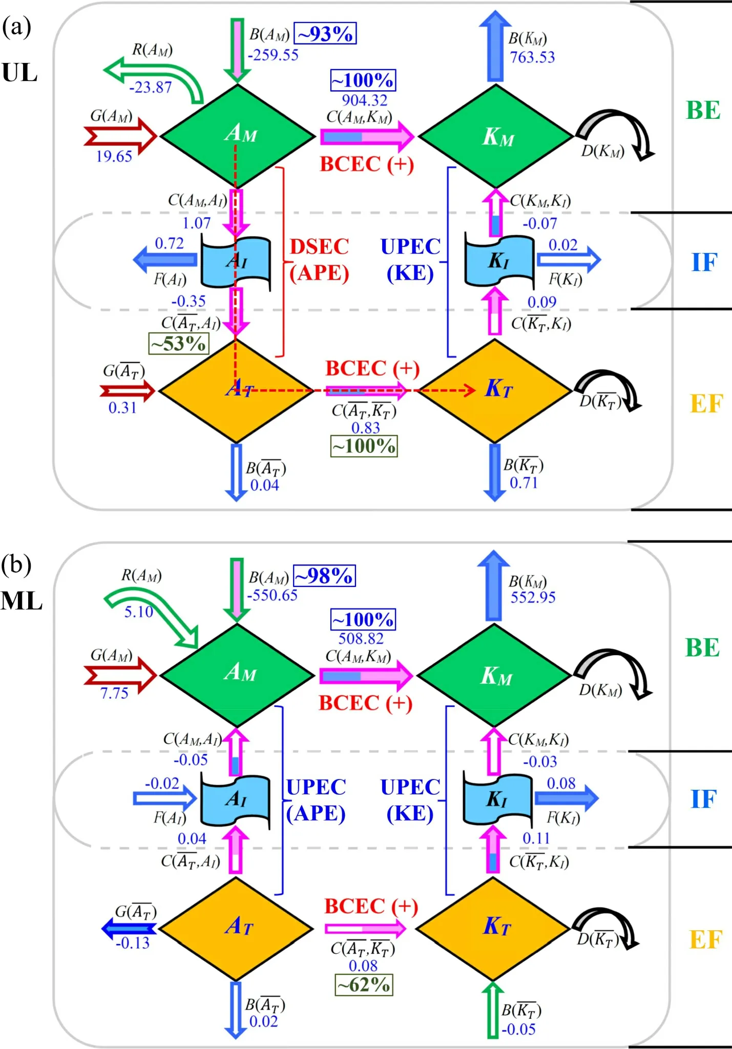
Fig. 6. Vertical integral of the key-region averaged budget terms of Eqs. (1)–(4) (blue values,units: W m–2) among the upper layer (200–450 hPa) (a) and the middle layer (450–700 hPa)(b). Blue percentages (within small blue boxes) indicate the contributions of the most favorable factors for the maintenance of the background environment (i.e., AM and KM). Green percentages (within small green boxes) indicate the contributions of the most favorable factors for the maintenance of the eddy flow (i.e., AT and KT). Green arrows show net-import transport, blue arrows show net-export transport, purple arrows show conversions between different types of energies, dark red arrows show diabatic production/extinction of APE,curved arrows show the effects of the dissipation terms, and the red dashed curved arrows outline the energy-cascade-related paths that provided energy to KT. The dominant factor for the maintenance/dissipation of each energy is shaded with light purple/blue. The purple arrows may be shaded in two colors because the conversions that they represent are dominant factors for two types of energies. UL = upper layer; ML = middle layer; BE = background environment; IF = interaction flow; EF = eddy flow; BCEC = baroclinic energy conversion,where “+” and “–” represent the release and production of APE, respectively. DSEC/UPEC =downscale/upscale energy cascade.

As mentioned above, for the middle and upper troposphere, energy features within the KR can effectively represent those within the northern and southern sections. In contrast, for the lower troposphere, the northern and southern sections should be analyzed separately. In order to show the energy budgets at various vertical layers, three equal-weight layers are defined: the upper layer (200–450 hPa), the middle layer (450–700 hPa), and the lower layer (700–950 hPa).Using ERA5 reanalysis data, each term in Eqs. (1)–(4) is first calculated at every grid point and then averaged horizontally within the KR, the northern section, and the southern section, respectively. After that, the corresponding results are integrated vertically in the upper, middle, and lower layers,respectively, to represent the overall energy features within a specified region at a selected layer.

4.2.Energy paths that sustained the background environment

The upper-tropospheric divergent wind field (Fig. 3a),middle-tropospheric warm advection (Fig. 3b), and lower-tropospheric southwest monsoonal wind (Fig. 3c) provided a favorable background environmentbThe wind and temperature fields of the background environment can be effectively represented by KM and AM, respectively (Murakami,2011; Fu et al., 2018).for the torrential rainfall. As Fig. 6a shows, upper-tropospheric KMwas maintained through the baroclinic conversion [i.e., C(AM, KM)] of AMto KM, which sustained the anticyclonic divergent wind field.As seen from Fig. 6b, AMand KMin the middle layer were mainly sustained via three-dimensional transport of AM[i.e.,B(AM)] and baroclinic conversion, respectively. The former maintained the temperature gradient (temperature decreased towards the southeast), and the latter sustained the westerly wind. These features contributed to the maintenance of middle-tropospheric warm advection. KMin the lower troposphere was sustained via baroclinic conversion of AMto KM(not shown), which maintained the strong southwest monsoonal wind.

4.3.Energy paths that maintained eddy flow

In the lower layer, the energy paths that supported KTwithin the northern and southern sections notably differed from each other (cf., Figs. 7a and b). For the northern section, its dominant energy path was the baroclinic energy conversion of ATto KT[i.e.,], which accounted for ～80% of the energy supply for KT(Fig. 7a). This conversion occurred mainly due to a direct thermal cycling (purple ellipse in Fig. 2a) associated with the front in the northern section, during which relatively warm air ascended along the tilted front while relatively cold air descended. This resulted in a net lowering of the air-column’s barycenter and an increase in its wind speed. The remaining 20% energy supply for KTwas contributed by three-dimensional transport of KT[i.e.,] (Table 2). Of this, the transport by the southwesterly wind through the northern section’s southern boundary made the largest contribution (not shown). Decomposing this transport into the FP and SP shows that the transport by the background environment (i.e., FP) made a larger contribution (～58%) than eddy flow (i.e., SP).

For the lower layer of the southern section, two energy paths supplied energy to the torrential-rainfall-producing eddy flow (Table 2). Three-dimensional transport of KT[i.e.,was dominant, which accounted for ～72% of the energy supply for KT(Fig. 7b). Of this, transport of KTby southwesterly wind through the southern boundary of the southern section contributed the largest amount. Further decomposition of this transport shows that the background environment (i.e., FP) and eddy flow (i.e., SP) accounted for ～68% and ～32%, respectively. The second energy path (～28% in contribution) consisted of two processes (red dashed line with arrowhead in Fig. 7b): (i) the baroclinic energy conversion of AMto KMand (ii) the downscale energy cascade of KE from KMto KT. There is a sharp contrast between the baroclinic energy conversion within the northern and southern sectionsin Figs. 7a and b]; as for the latter, there was a conversion of KTto AT. As seen from Fig.2b, the southwesterly wind decelerated within the southern section, which led to convergence and lifting of the air-column’s barycenter. This enhanced the eddy flow’s APE and reduced its KE, resulting in the baroclinic energy conversion of KTto AT.

In the upper layer, the energy path that supplied energy to KTwithin the KR contained two processes (red dashed line with arrowhead in Fig. 6a): first, AMwas converted into ATthrough a downscale APE cascade; then ATwas converted to KTvia baroclinic energy conversion. This was the only energy source for the upper-tropospheric eddy flow (Table 2),whereas other terms mainly acted to reduce KT(Fig. 6a).

In the middle layer, two energy paths maintained KT(Fig. 6b). The baroclinic energy conversion of ATto KTcontributed ～62% of the total energy income for KTwithin the KR. This conversion was closely related to the middle-tropospheric baroclinic shortwave trough (Fig. 3b). The second energy path was the three-dimensional transport of KT[i.e.,, which accounted for ～38% of the total energy income for KTwithin the KR (Fig. 6b). Further analysis indicates that westerly winds in the background environment(mainly through the key region’s western boundary) dominated this transport (Table 2).

Table 2. Three-dimensional energy paths that sustained KE of the torrential-rainfall-producing eddy flow (KT) within different regions[symbols “→” and “←” denote the directions of energy conversion; percentage below a vector denotes its relative contribution; the wind that had dominant effect for B() is shown within parentheses to the right] and their energy cascade features (their main effects are shown within parentheses). BE = Background environment.

Table 2. Three-dimensional energy paths that sustained KE of the torrential-rainfall-producing eddy flow (KT) within different regions[symbols “→” and “←” denote the directions of energy conversion; percentage below a vector denotes its relative contribution; the wind that had dominant effect for B() is shown within parentheses to the right] and their energy cascade features (their main effects are shown within parentheses). BE = Background environment.

4.4. Contributions of different signals in the background environment

This section discusses the contributions of different background environment signals in maintaining the eddy flow’s wind field (in terms of KT) at the lower layer. The Lanczos band-pass filtering technique (Duchon, 1979) is utilized to separate QWO, QBO, and ISO (Fig. 4c) from the background environment (using the hourly ERA5 reanalysis data during the period from 1 April to 1 October). We define the rest of the background environment after removing QWO, QBO,and ISO as the remaining background environment (RBE).As seen from Fig. 4b, the RBE mainly contained signals that had larger periods than ISO. This is confirmed in Fig.8d, which shows that the RBE consisted of the typical situation of a summer monsoonal season (Ding, 1994; Zhao et al., 2004). Comparisons among QWO, QBO, and ISO (cf.,Figs. 8a–c) indicate that QBO had the largest intensities of geopotential height, temperature, and wind filed, whereas,QWO had the smallest intensities. Overall, QWO exhibited a vortex structure around the KR, causing weak perturbations of temperature and wind (Fig. 8a). QBO exhibited a transversal trough structure around the KR (Fig. 8b), with strong northeasterly and westerly wind perturbations appearing in its northern and southern parts, respectively. Temperature perturbations were strong within the northern section, corresponding to the front in this region. ISO exhibited a ridge structure around the KR (Fig. 8c), and its associated wind and temperature perturbations were weak.

Fig. 7. The same as Fig. 6, but for the northern section of the lower layer (950–700 hPa) (a)and southern section of the lower layer (b), where the red percentages (within small red boxes)indicate the contributions of the second most favorable factors that sustained KT. NS =northern section; SS = southern section.

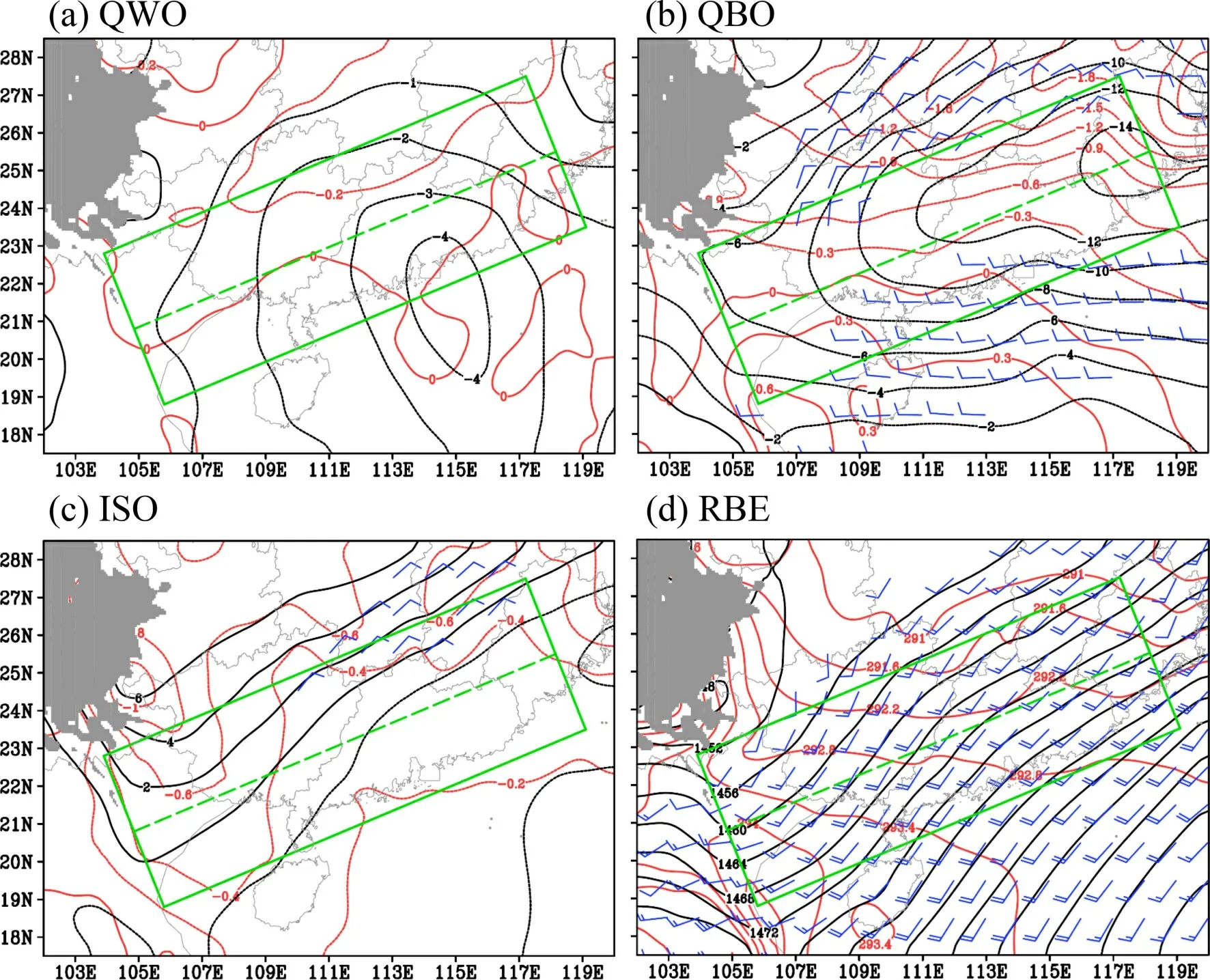
Fig. 8. The 850-hPa geopotential height (black contours, units: gpm), temperature (red contours, units: K), and wind above 3 m s–1 (a full wind bar is 4 m s–1) of QWO (a), QBO (b), ISO (c), and the RBE (d). Grey shading marks the terrain above 1500 m, and the green tilted box shows the key region, with a green dashed line dividing it into the northern and southern sections.

As Table 2 shows, for the eddy flow in the lower layer of the northern section, scale interactions were not a dominant factor for its sustainment; instead, baroclinic conversion in eddy flow was the governing factor, which accounted for ～80% of its energy source. In contrast, for the eddy flow in the lower layer of the southern section, scale interactions dominated its maintenance (～77% contribution) via two processes: a downscale energy cascade of KE (28% contribution) and a three-dimensional transport of KTby the background environment wind field (i.e., FP; 49% contribution).The FP is further decomposed to compare the transport of KTby respective QWO, QBO, ISO, and RBE wind fields. It is found that the transport due to the RBE wind field (i.e.,the southwest monsoonal wind) had the largest intensity(Fig. 9d), whereas, that due to the QWO wind field was weakest (Fig. 9a). Overall, in the lower layer of the southern section, the transport of KTby the RBE contributed the largest proportion at over 60% (Table 3); the contributions of QBO and ISO (Figs. 9b and c) were also notable and accounted for 21.3% and 14.6%, respectively (Table 3). In contrast,QWO showed the smallest contribution to the transport of KT(4.1%).

The energy cascade terms of KE in the lower layer are shown in Fig. 10a. A configuration of negative C(, KI)with positive C(KM, KI) is notable in the southern section,whereas, in the northern section, negative C(, KI) is not obvious. This is a direct reason for why only the southern section exhibited a clear downscale KE cascade. In order to compare the contributions of different background environment signals, energy cascade terms of KE due to respective QWO,QBO, ISO, and RBE are calculated. As Figs. 10b–d show,within the southern section, C(, KI) generally had a larger absolute value than C(KM, KI). This means that QWO,QBO, and ISO were more important in determining C(,KI) (i.e., the conversion between eddy flow KE and interaction flow KE) than C(KM, KI) (i.e., the conversion between background environment KE and interaction flow KE). Positive C(, KI) (i.e., the conversion of KTto KI) due to the RBE(Fig. 10f) canceled out the QWO+QBO+ISO associated negative C(, KI) within the northern section (Fig. 10e), which is the key reason why no obvious downscale KE cascade appeared in this section.

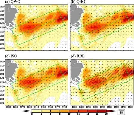
Fig. 9. The 850-hPa KT (shading; J kg–1) and the transport of KT (vectors, units: W m kg–1) by the wind field of QWO (a), QBO (b), ISO (c), and the RBE (d). Grey shading marks the terrain above 1500 m, and the green tilted box shows the key region, with a green dashed line dividing it into the northern and southern sections.

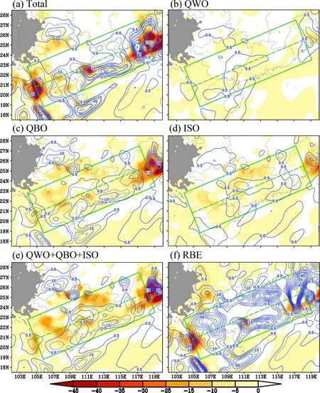
Fig. 10. Terms C(KM, KI) (solid blue; 10–5 W kg–1) and C( , KI) (shading; 10–5 W kg–1) calculated by the total background environment (a), QWO (b), QBO (c), ISO (d), QWO+QBO+ISO (e), and the RBE (f). Grey shading marks the terrain above 1500 m, and the green tilted box shows the key region, with a green dashed line dividing it into the northern and southern sections.

Overall, for the lower layer of the southern section, the RBE dominated term C(KM, KI), which made a contribution of 71.7% (Table 3). For term C(, KI), QBO exhibited the largest contribution (39.3%), which is 8% higher than that of the RBE. This indicates that both the monsoonal wind (i.e., the RBE) and perturbations in the monsoonal wind (i.e.,QWO, QBO, and ISO) were crucial to the downscale KE cascade, whereas their relative importance was different for terms C(KM, KI) and C(, KI).

Table 3. Contribution (units: %) of different BE signals in the transport of KT (i.e., FP), and KE cascade processes at the lower layer of the southern section.

5.Conclusion and discussion

In this study, a torrential rainfall event is found to be directly induced by eddy flow, which is embedded in a favorable background environment. Clarifying the respective variation mechanisms of the torrential-rain-producing eddy flow and its background environment and exploring their interactions are key to promoting the understanding of torrential rainfall events. This study provides a general methodology for investigating torrential rainfall energetics and applies that methodology to quantitatively solve the above three problems. The proposed methodology is conducted on a persistent torrential rainfall event in the pre-summer rainy season of 2017, during which concurrent frontal and warm-sector precipitation appeared. Horizontal distribution features of this rainfall event are consistent with those derived from a 12-yr statistic of the torrential rainfall events over South China(Wu et al., 2020a); frontal heavy rainfall associated with fronts or shear lines mainly occurs over inland regions of South China, whereas warm-sector heavy rainfall is mainly observed in coastal areas. Based on the budgets of energetics derived from the selected case, we provide the first physical image of the energetics of this type of precipitation. For the first time, key similarities and differences between the warm-sector and frontal rainfall are shown from the perspective of energetics.

Similarities and differences between the frontal and warm-sector heavy rainfall are notable and consistent with the 12-yr statistic shown by Wu et al. (2020a). In this study,we discuss the same topic in terms of energetics. It is found that similarities between the concurrent frontal and warm-sector rainfall for the chosen case mainly appeared in the upper and middle troposphere, where the upper-tropospheric divergent background environment wind field was maintained primarily by baroclinic energy conversion and the middle-tropospheric background environment warm advection was sustained primarily through three-dimensional transport and baroclinic energy conversion. Fundamental differences between the concurrent frontal and warm-sector rainfall mainly appeared in the lower layer, where the eddy flow APE and KE both had maximum values. For the warm-sector rainfall,its associated eddy flow maintained its strong KE mainly via two mechanisms: a three-dimensional transport of KTby the southwest monsoonal wind and a downscale KE cascade from the background environment. This means that from the viewpoint of energy sources, improving the forecasting of the southwest monsoonal wind in the lower latitudes and the large-scale background environment over South China (particularly in the lower troposphere) is of key importance to the forecasting of warm-sector torrential rainfall. For the frontal rainfall, its associated eddy flow was mainly sustained through a baroclinic energy conversion in the eddy flow, corresponding to the direct thermal cycling of the front. Overall, scale interactions were a dominant factor for sustaining the eddy flow that produced the warm-sector rainfall,whereas for the frontal rainfall, scale interactions were only of secondary importance. Calculations indicate that the RBE

wind field (i.e., the southwest monsoonal wind) made the largest contribution in the scale interactions for sustaining the warm-sector-rainfall-associated eddy flow in the lower layer; the QBO wind field acted as the second most dominant factor.

In this event, the region with lower-level KTabove 7 J kg–1(i.e., eddy flow was strong) mainly stretched along the coastline (Fig. 1a), which was similar to the distribution of the cloud area with a TBB (temperature of black body) temperature below –52°C (not shown). The northern section(where mean terrain height is higher than that of the southern section) had larger lower-level KTthan the southern section(Fig. 5d). This means that the inhomogeneous underlying surface of South China (e.g., topography and land–sea contrast)was influential on the distribution of eddy flow KE, since it acts as a common trigger for warm-sector rainfall (Xu et al.,2012; Chen et al., 2015, 2016). A southwesterly low-level jet was notable in this event (not shown) and transported KTat lower latitudes into the. It was the dominant factor for the sustainment of the eddy flow that induced the warm-sector torrential rainfall (Table 2). This is consistent with the findings of Du and Chen (2018, 2019a, b), who analyzed a similar torrential rainfall event with concurrent frontal and warm-sector precipitation and found that a boundary layer jet at 925 hPa, which occurred over the northern region of the South China Sea, played a key role in triggering and maintaining the warm-sector rainfall. Although the torrential rainfall event used in this study is typical, it is still limited in its ability to reflect the general energy features of the warm-sector torrential rainfall. Since this study provides a general energetics methodology for investigating torrential rainfall, we recommend conducting further analyses on more warm-sector torrential rainfall cases in the future. This will contribute to reaching a more comprehensive understanding of warm-sector torrential rainfall in terms of energetics.

Acknowledgements.The authors would like to thank ECMWF and NCAR for providing the data used in this study. This research was supported by the National Key R&D Program of China (Grant No. 2018YFC1507400), and the National Natural Science Foundation of China (Grant Nos. 42075002 and 42030610).