Tingting Ji(冀婷婷)， Naiqiao Pan(潘乃桥)， Tian Chen(陈天)， and Xiangdong Zhang(张向东)

Key Laboratory of Advanced Optoelectronic Quantum Architecture and Measurements of Ministry of Education，Beijing Key Laboratory of Nanophotonics&Ultrafine Optoelectronic Systems，School of Physics，Beijing Institute of Technology，Beijing 100081，China

Keywords: quantum search，the joined complete graph，quantum walk，many vertices

1. Introduction

Although the Grover algorithm has achieved great success in the quantum search problem， the direct application of this algorithm in physical databases，e.g.，the graph structure，cannot work well.In many circumstances，the relations among these physical databases are described by the Hamiltonians.Some efforts have been devoted to applying the Grover algorithm to such databases，but the evolutions governed by these Hamiltonians cannot be easily designed as the requirements of the Grover algorithm. In order to realize the fast quantum search in physical databases described by the Hamiltonians，Childs and Goldstone proposed a graph-based continuoustime quantum walk search algorithm.[11]Random walk is widely employed in designing the classical algorithms，so it is natural to extend the algorithm of random walk from classic to quantum version.The studies of the quantum algorithms based on the graphs have attracted lots of attention.[12–19]Quantum algorithms based on continuous-time quantum walks have revealed an exponential acceleration that surpasses any classical algorithm in solving a certain black-box problem，and can provide a corresponding framework for designing new algorithms， modeling quantum transmission and state transition problems.[20–33]Considering that the graph structure can represent different connections between the vertices，the quantum search algorithms on the graph are also very important. The viewpoint about the success of searching the vertices in the graph depending on the connectivity in the graph lasted over one decade.[34，35]Recent researches point out that through the design of the jumping rate between the adjacent vertices in the graph，the quantum search of the target vertex can be realized in the low-connectivity graphs， which exhibits the quantum advantage over the classical algorithm.[36–40]In these works，the researchers concern about the searching one vertex and such vertex does not locate at the“specific”position(i.e.，not on the positions with different connectivity).

In the following， we firstly provide different cases in which the target vertices locate at different positions.Then，we derive and show the general expressions for quantum search in these cases. Graphs with different numbers of vertices are presented to verify the success of quantum search. We conclude at the end of this paper.

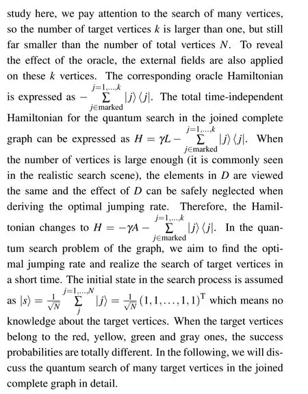
2. General descriptions of the joined complete graph

The joined complete graph is addressed below (Fig. 1)，which containsNvertices. There areN/2 vertices in the left complete graph and the otherN/2 vertices belong to the right complete graph. The degree ofjth vertex(deg(j))is defined as the number of connecting vertices.So it is clear that the vertices in red， blue， gray and white have the same degrees， but the vertices in yellow and green have the same degrees，which are not the same as above.

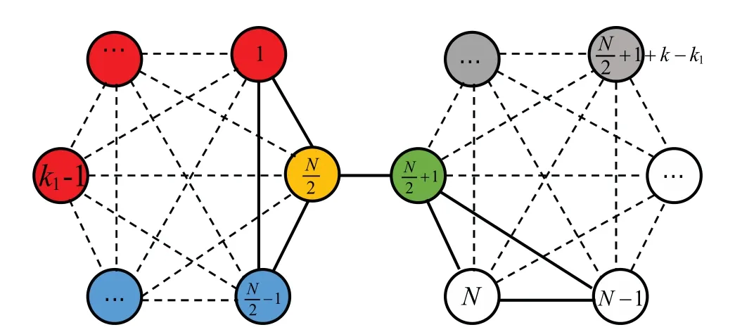
Fig.1. The schematic representation of the joined complete graph. The vertices in red，blue，gray and white have the same degree deg(j). The yellow(green)vertex that connect to the other complete graph has different degree. In our discussions， the target vertices may be the red，gray，yellow and green ones. The detailed study is addressed below.

3. The quantum search of many vertices in the joined complete graph

The positions of target vertices can be grouped into several different cases. In the below，we will provide the derivation of optimal jumping rate in each case and verify the success of the quantum search of these target vertices. As shown in Fig.1，the joined complete graph is composed by one complete graph in the left and the other complete graph in the right.Therefore，the successful search with the maximum probability relies on the distribution of the target vertices. If target vertices are all located at the left or right complete graph，the successful search is defined as the search probability of target vertices being very close to 1/2.This value 1/2 results from the low connectivity between the left and right complete graphs.The evolution of search starts from the equal superposition of all vertices. In the search process， when the target vertices are only located on one complete graph， the probabilities on the other complete graph cannot fully flow into the adjacent complete graph by going through the only one connection between these two complete graphs. The simplest case is finding only one vertex in the joined complete graph.[35]As the target vertex is only on one of the complete graphs， the successful search is defined with the probability of finding the target vertex as 1/2. In comparison，if some target vertices are located at the left and the others are located at the right complete graph，the successful search is defined as the search probability of target vertices being very close to 1. In this scenario，the probabilities on each complete graph are accumulated to the target vertices on the corresponding graph during the search process.

In realistic conditions， the number of target verticeskis commonly far smaller than the number of total verticesN. In our discussion， we assume such condition is satisfied in all cases.

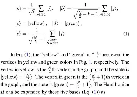
3.1. All the target vertices are red ones

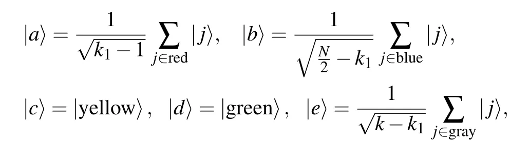
Here，we study the case whenktarget vertices are all red ones. In this case， all the target vertices are located on the left complete graph. All vertices are grouped according to the connectivity on the graph. The target vertices are grouped together，and the other vertices can be grouped based on the connection with the target vertices and the location on the graph.The reason to group all vertices into different categories is for finding the optimal value ofγconveniently. The details are addressed below. In this case，the vertices in gray and white in the right complete graph can be seen as the vertices possessing the same properties. According to the method shown in Ref.[35]，we can group theNvertices into five categories as

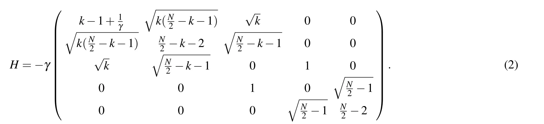
When the number of target verticeskis commonly far smaller than the number of total verticesN，we simplifyHto

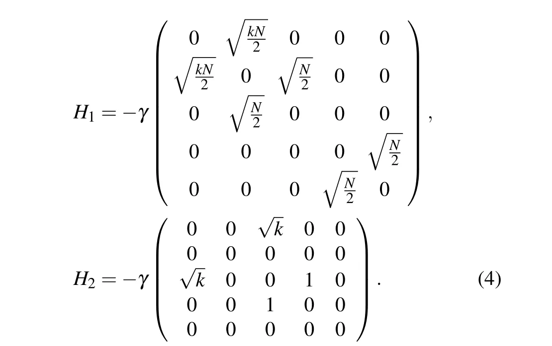
WhenNis large enough，the elements inH0are far larger than those inH1andH2，and the elements inH1are far larger than those inH2. So the effect fromH2can be neglected safely.Considering there is no knowledge about target vertices at the beginning，the initial state of quantum search is

3.2. The k1 target vertices in red and (k-k1) target vertices in gray

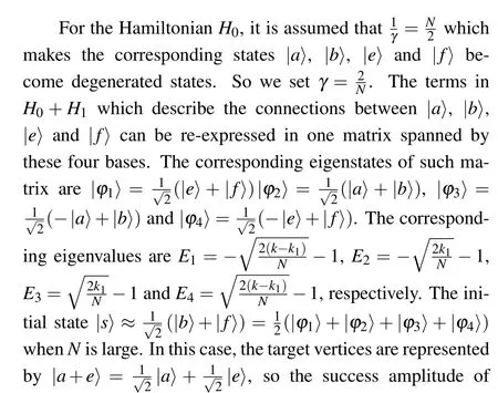
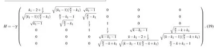
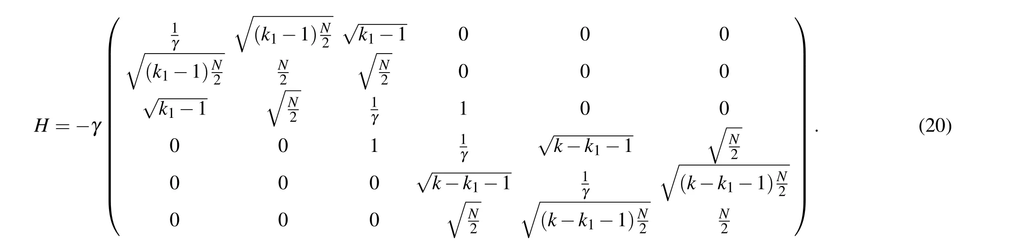
When the target vertices are not all in red， the situation will be different. For the second case，it is assumed that there arek1target vertices in red and(k-k1)target vertices in gray.In this case， the vertices in the joined complete graph can be grounded into six categories in Eq.(6)as

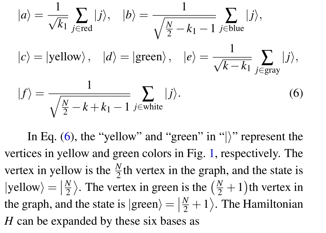
When the number of target verticeskis commonly far smaller than the number of total verticesN，we simplifyHto

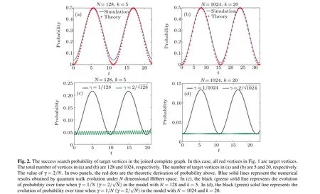
Fig. 3. The success search probability of target vertices in the joined complete graph. In this case，k1 target vertices in red and(k-k1)target vertices in gray. The total number of vertices in(a)and(b)are 128 and 1024，respectively.The number of target vertices in red(gray)in(a)and(b) are 5 (5) and 10 (10)， respectively. The value of γ =2/N. In two panels， the red dots are the theoretic derivation of probability above.Blue solid lines represent the numerical results obtained by quantum walk evolution under N dimensional Hilbert space.

3.3. The(k-1)target vertices in red and one target vertex in yellow

In this case，the situations are different from above. One of the target vertices locates at the position in the graph possessing different connectivity with the other target vertices.Here we assume there are (k-1) target vertices in red and the remaining one target vertex in yellow. So the vertices in gray and in white can be viewed as one type of vertices having the same properties. We can group the total vertices into five categories as follows:

When the number of target verticeskis commonly far smaller than the number of total verticesN，we simplifyHto

As reflected from these two panels， the numerical and theoretical results agree with each other well. For case C with the target vertices locating at the left complete graph， the maximum searching probability reaches 1/2 with the optimal jumping rate，which means the successful search has been realized.Compared with Figs. 4(a) and 4(b)， we can find that the difference between the numerical and theoretical results becomes smaller when the number of vertices is larger. When the total number of vertices isN=128(1024)， the maximum success probability in finding these vertices is achieved at the first time att=6.28(17.77).

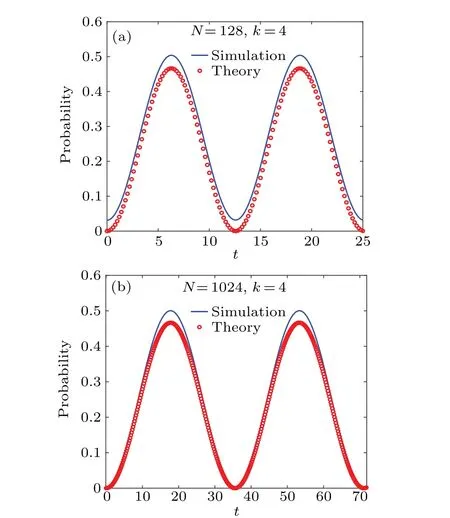
Fig. 4. The success search probability of target vertices in the joined complete graph. In this case， (k-1) target vertices in red and the remaining target vertex in yellow. The total number of vertices in(a)and(b)are 128 and 1024，respectively. The number of target vertices in red in(a)and(b)are both k-1=3. The value of γ =2/N. In two panels，red dots are theoretic derivations of probability above. Blue solid lines represent numerical results obtained by quantum walk evolution under N dimensional Hilbert space.

3.4. The (k1-1) target vertices in red， one in yellow and(k-k1)target vertices in gray

Here，the target vertices are distributed into two complete graphs and one of them locates at the position with different connectivity. There are(k1-1)target vertices in red，one target vertex in yellow，and(k-k1)target vertices in gray.So we can group these vertices into six categories

When the number of target verticeskis commonly far smaller than the number of total verticesN，we simplifyHto

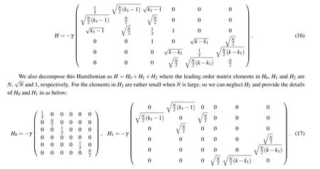
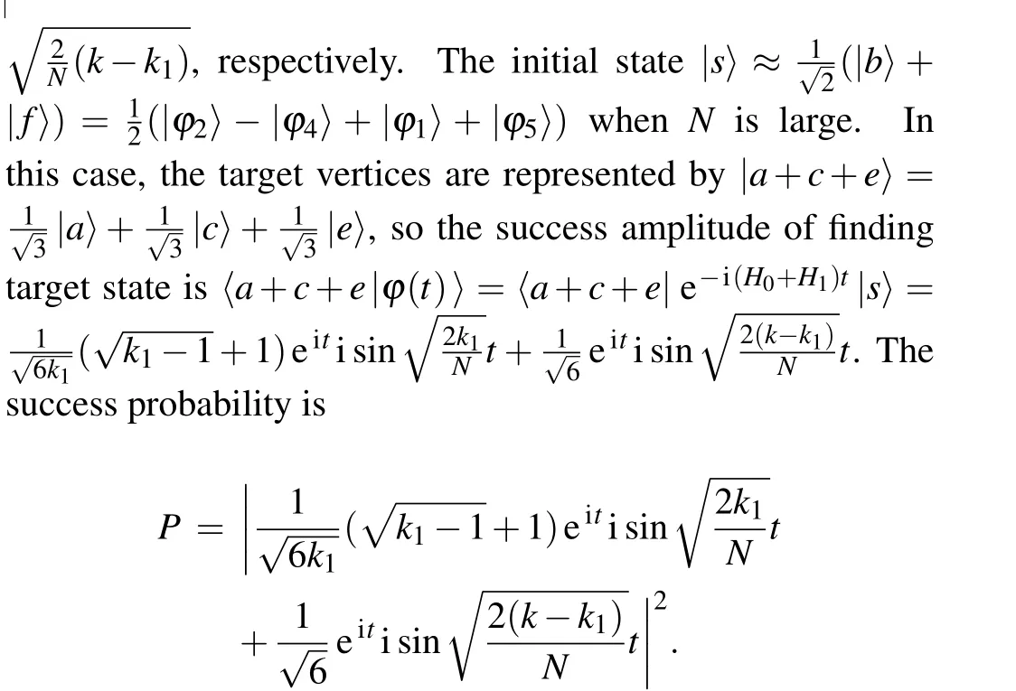
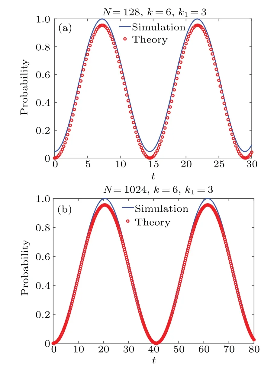
Fig. 5. The success search probability of target vertices in the joined complete graph. In this case， (k1-1)target vertices in red， one target vertex in yellow and(k-k1)target vertices in gray. The total number of vertices in(a)and(b)are 128 and 1024，respectively. The number of target vertices in red (gray) in(a)and(b) are both 2 (3). The value of γ=2/N.In two panels，the red dots are the theoretic derivation of probability above. Blue solid lines represent the numerical results obtained by quantum walk evolution under N dimensional Hilbert space.

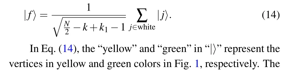
3.5. The (k1-1) target vertices in red， one in yellow， one in green，and the remaining(k-k1-1)in gray

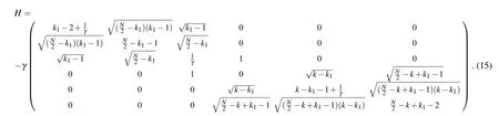
Here，we consider another case that the target vertices locate at each complete graph. There are(k1-1)target vertices in red，one in yellow，one in green，and(k-k1-1)target vertices in gray. All of the vertices can be grouped into six categories as

When the number of target verticeskis commonly far smaller than the number of total verticesN，we simplifyHto

In Fig.6， we provide the numerical(blue lines)and theoretic (red dots) results. In this case， the target vertices are(k1-1)in red，one in yellow，one in green and(k-k1-1)in gray. As revealed from these two panels， the numerical and theoretic results coincide with each other well. For case E with the target vertices locating at two complete graphs， the maximum searching probability reaches 1 with the optimal jumping rate，which means the successful search has been realized. Compared with Figs. 6(a) and 6(b)， we can find that the difference between the numerical and theoretical results becomes smaller at the beginning of the evolution when the number of vertices is larger.When the total number of vertices isN=128(1024)， the maximum success probability in finding these vertices is achieved at the first time att=7.2(17.8).

In the following，we provide a table to summarize the results of the above derivation.

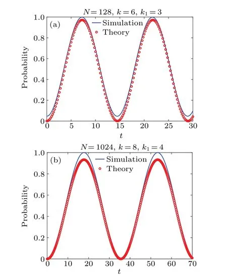
Fig. 6. The success search probability of target vertices in the joined complete graph. In this case， (k1-1)target vertices in red， one target vertex in yellow， one in green and (k-k1-1) target vertices in gray.The total number of vertices in (a) and (b) are 128 and 1024， respectively. The number of target vertices in red (gray) in (a) and (b) are 2 and 3 (2 and 3)， respectively. The value of γ =2/N. In two panels，the red dots are the theoretic derivation of probability above. Blue solid lines represent the numerical results obtained by quantum walk evolution under N dimensional Hilbert space.

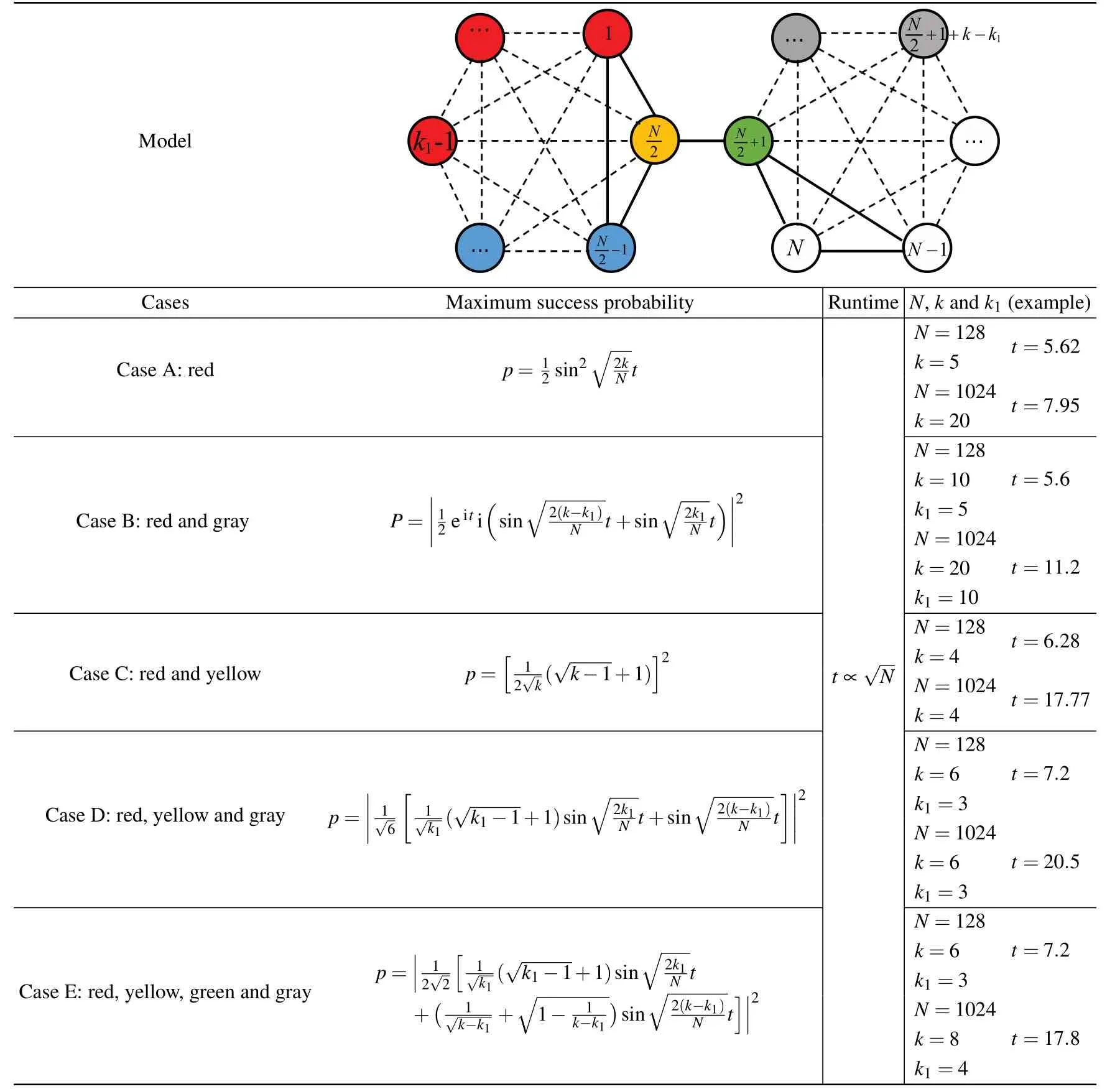
Table 1. The quantum search on the joined complete graph. The colors for the target vertices are shown in cases A–E.

4. Conclusion

Acknowledgements

Project supported by the National Key R&D Program of China (Grant No. 2017YFA0303800) and the National Natural Science Foundation of China (Grant Nos. 91850205 and 11974046).