Lin-ge Li，Zhonghuai Hou✉

1 Hefei National Laboratory for Physical Sciences at the Microscale & Department of Chemical Physics, University of Science and Technology of China, Hefei 230026, China

Abstract Liquid—liquid phase separation (LLPS) has proved to be ubiquitous in living cells, forming membraneless organelles (MLOs) and dynamic condensations essential in physiological processes. However,some underlying mechanisms remain challenging to unravel experimentally, making theoretical modeling an indispensable aspect. Here we present a protocol for understanding LLPS from fundamental physics to detailed modeling procedures. The protocol involves a comprehensive physical picture on selecting suitable theoretical approaches, as well as how and what to interpret and resolve from the results. On the particle-based level, we elaborate on coarse-grained simulation procedures from building up models, identifying crucial interactions to running simulations to obtain phase diagrams and other concerned properties. We also outline field-based theories which give the system's density profile to determine phase diagrams and provide dynamic properties by studying the time evolution of density field, enabling us to characterize LLPS systems with larger time and length scales and to further include other nonequilibrium factors such as chemical reactions.

Keywords Liquid—liquid phase separation, Theoretical modelling, Coarse-grained simulation

INTRODUCTION

Cellular compartmentalization plays an essential role in biological function, from providing spatiotemporal organization of cellular materials to regulating biochemical reactions. It is recently proved that liquid—liquid phase separation (LLPS) is ubiquitous in cells and often underlies the formation of some compartments, either forming organelles that lack delimiting membranes (namely membraneless organelles) such as Cajal bodies and nucleoli or generating dynamic biomolecule condensates facilitating physiological processes (Boeynaemset al.2018; Brangwynneet al. 2009, 2015; Hymanet al.2014; Molliex et al.2015). While experiment discoveries are mounting on the significant role LLPS plays in diverse cell functions, some underlying mechanisms remain challenging to determine experimentally, considering the disordered nature of such assemblies. Consequently, it is of great significance for theoretical and computational approaches to assist in unraveling various biophysical phenomena. In this regard, there have been many excellent theoretical works on biological condensation with separate modeling scales and methods aiming at different systems (Alshareedah et al. 2020; Bracha et al.2019; Chang et al. 2017; Gasior et al. 2019; Guillén-Boixet et al. 2020; Monahanet al. 2017; Nott et al.2015; Wei et al. 2020). Nevertheless, a comprehensive physical picture is still required for those who want to get started on a theoretical interpretation.

In this protocol, we aim to present a conceptual framework on selecting suitable methodology and what to interpret and answer from the simulation or theoretical results, which is organized as follows. We briefly introduce the general physical picture of phase separation and how it is applied in biophysical studying. Then we detail the major theories and methodologies required for a simulation or analytical studying, with related examples specifically described and discussed. Finally, we discuss other essential aspects for biomolecular condensates and future research routes.

A primer on biophysical phase separation

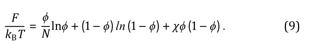
LLPS in cells is a collective process that generally involves multiple components with complex interactions, during which the biomolecules can condense into the formation of a dense phase coexisting with a dilute one. From the perspective of equilibrium statistical physics, such biophysical phenomenon is governed by the change of free energy F, which consists of enthalpic and entropic terms:

For phase separation to occur, it requires an evident decrease in free energy from mixing to demixing states,i.e., ∆F <0, which corresponds to a negative change in enthalpy (∆ H<0) or positive change in entropy(∆ S>0) as the driving force. Decreasing enthalpy in biosystem mainly originates from various types of electrostatic interactions, including hydrogen bonds as in between water, proteins and nucleic acids;charge—charge interactions between charged amino acids or nucleotide nucleic acids; and π interactions in which sp groups or aromatic rings can interact with each other or cations. Regarding entropy, a major aspect is a conformational heterogeneity, as evidence is mounting that many of those phase-separating proteins are disordered or contain intrinsically disordered regions (IDRs) (Burkeet al. 2015). Another typical example of entropy effect is due to hydrophobic contact ubiquitous in water, in a sense that possible configurations of hydrogen bonding may be restricted at the nonpolar surface of biomacromolecules, which tend to be compacted to minimize the water molecules participating in a solvation shell and maximizes entropic solvation free energy (Huang and Chandler 2002) (Fig. 1A).

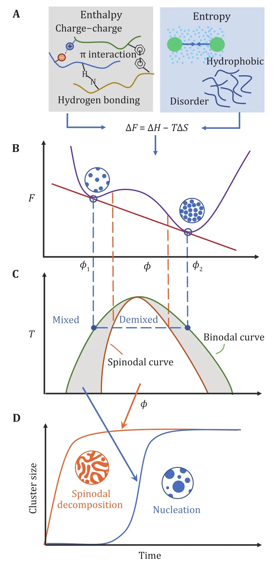
Fig. 1 Thermodynamics and dynamics of equilibrium phase separation. A Driving forces in LLPS, some enthalpic and entropic effects are listed. B Free energy profile. F is free energy, ϕ is an order parameter such as volume fraction. With two local minima in the free energy curve, the system can phase separate into a dilute phase with volume fraction ϕ1 and dense phase of ϕ2. C Phase diagram with regions of mixed and demixed phases delineated by the binodal curve. The spinodal curve separates the stable and metastable regions. D Two types of dynamic mechanisms on the cluster growth process, namely spinodal decomposition and nucleation

General framework of selecting theoretical method

In the context of the high degree of complexity in a phase separation system, atomistic simulations using quantum mechanics or atomic molecular dynamics(MD) would usually be severely limited in scope for a given computational budget. Nevertheless, such detailed resolution can be useful in obtaining parameters for larger scales (Murthy et al. 2019),capturing inter-residue interaction potentials (Zerze et al. 2015) and providing structural characteristics of single protein conformations (Conicella et al. 2016). To reduce the level of complexity in particle-based simulation, coarse-graining (CG) is indispensable for constructing practicable protocols, the degree of which can vary from multiple beads per monomer to single bead per molecule (Ruff et al. 2019). However,considering the tradeoff between efficiency and accuracy, the choice of coarse-grained resolution should be question-specified, capturing the major physics as well as deploying practical computational resources. Detailed coarse-grained simulation methods will be discussed in the following section.

SUMMARIZED PROCEDURE

Select a suitable theoretical method

1Select a qusestion-specified method. On the basis of accuracy and scale required, choose the particlebased method (Steps 2—8) or the field-based method (Steps 9—12).

Perform particle-based MD simulation

2Set up system conditions. Choose proper simulation units, dimensions, boundary conditions and the dynamic equation for MD simulation.

3Build up a coarse-grained model. Select the residuebased, rigid body or CG particles to describe your molecules.

4Generate initial configuration of multiple molecules in simulation box to reach target concentration.

5Identify crucial interactions and parameterization.

6Run simulations. Warm-up first to avoid extremely unreasonable initial configurations, and then run certain steps until the system reaches equilibration.

7Proceed simulations under different conditions to obtain phase diagrams. Apply slab method for T—c phase diagram.

8Obtain trajectories and analyze simulation results.

Perform field-based simulation

9Obtain suitable free energy functional that characterize crucial interactions.

10 Determine unit volume, system size and initialize density profile.

11 Employ dynamic equations for each component and perform numerical simulation on dynamic evolution.

12 Obtain phase diagram, density evolution and other simulation results.

PARTICLE-BASED SIMULATION

Molecular dynamics (Step 2)

The general idea of molecular dynamics is to evolve positions of particles according to Newton's equations,which proceeds in the following steps: (1) Set up the initial configuration of model particles; (2) Integrate the particle positions and velocities at each time interval by numerically solving the classical equations of motion:

Building up a coarse-grained model (Step 3)

Coarse-graining means to treat several atoms as a large cluster that updates together. As described earlier, the coarse-grain level may vary from residue-based to the whole macromolecule and should be selected according to the given specified question. In addition, due to the many length- and time- scales involved in protein aggregation, different coarse-grained methods may be taken together to build up a multiscale model. Herein,we take the bacterial transcription factor protein GreB(Borukhov et al. 2005) as an example to discuss the following coarse-grain protocol, whose structure contains both disordered and folded regions (Fig. 2A).

Fig. 2 Modeling of proteins with separate levels of coarse grain demonstrated by GreB. A Schematic diagram of GreB structural domains and multiscale coarse-grained GreB structure. Detailed coarse-grained methods for each part are given in panels B, C and D. B Disordered regions are coarse-grained into residue-based beads, whose charge and interaction parameters are residue specified. In panels C and D, ordered regions are modeled as rigid bodies with coarse geometry according to crystal structures taken from the Protein Data Bank (PDB) and adapted to the model resolution. C CTD is modeled as a spherical rigid body with interaction sites. Locations determined from the charged residues(E, D, K and R) on the surface. D Coiled-coil region is represented as a dual-rod-like rigid body built with sphere particles outlining the structure for simulation benefit

The most common degree of coarse-grain for biomacromolecules is to treat each monomer (e.g.,amino acid or nucleotide) in the chain as a single interaction site, classifying particles according to residue types to capture sequence specificity(Dannenhoffer-Lafage and Best 2021; Dignonet al.2018). Since many of the phase-separating proteins are mainly or partially intrinsically disordered, such a residue-based model becomes an appropriate choice,allowing to highlight inter-residue charge effects as well as to reflect the flexibility of the disordered region.Therefore, we chose a residue-based model for disordered IDR of GreB (Fig 2B). Such models are particularly suitable for reproducing sequencedependent phase behaviors and predicting effects of mutations or PTMs of disordered proteins (Monahan et al. 2017).

However, such residue-based models fail to capture the secondary or higher structure of biomacromolecules,hence may no longer be appropriate for situations with folded domains. In this regard, the folded domain can be coarse-grained as a "rigid body" to preserve the structure feature as well as to reduce computation requirements (Dignon et al. 2018). As a simple situation,if the domains were near-spherical such as CTD of GreB,it can be approximately regarded as a single large sphere with interaction sites on the surface, also known as the"patchy colloid" model (Bianchi et al. 2011; Joseph et al.2021). Radius of the protein sphere can be obtained based on the radius of gyration or corresponding crystal structures taken from the Protein Data Bank (PDB),while locations and strengths of interaction sites can be adapted from crystal structures, NMR or bottom-up computations. Then the sites can be mapped onto the surface of the rigid body according to their relative positions (Fig. 2C, 2D). For other special-shaped structures such as the coiled-coil region in GreB, one can build up a rigid body that captures the geometry outline with a few CG sphere particles (Fig. 2A, 2D). In spite of an approximation, such a model can essentially capture the major physics with high simulation efficiency.

Further coarse-grained models may also be implemented depending on certain time- and lengthscales. For example, Guillén-Boixet et al. coarse-grained G3BP1 into two beads to capture NTF2 and RRM domain respectively, and RNA is coarse-grained so that each"bead" represents 8—10 nt (Guillén-Boixet et al. 2020).Falk et al. simulated chromosomes that are constructed from equally sized spherical monomers, with each of them representing 40 kb (Falk et al. 2019). Even the most ultra-coarse-grained model treating the entire IDP as a single sphere may be sufficient in specific issues(Bracha et al. 2019).

Identifying crucial interaction (Step 5)

Among many interatomic potentials that exist in a cellular environment, one should identify the essential physical variants responsible for LLPS and ignore the minor ones for simplicity.

Exclusive volume

First, we should always consider exclusive volume effects between all pairs of particles, commonly applied via Lennard-Jones (LJ) potential (Fig. 3A, blue line):

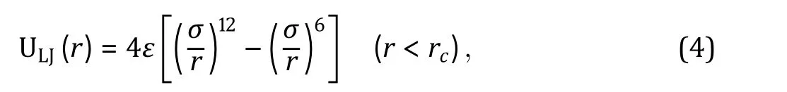
Bonded interactions

Bonded interactions between connecting neighbor particles can be described by harmonic springs (Fig. 3B):

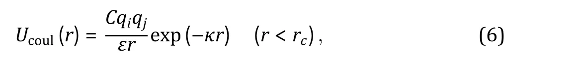
Electrostatic interactions

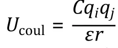
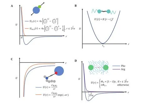
Fig. 3 Interaction potentials commonly applied in CG simulation. A Exclusive volume with L-J potential (blue line) and WCA potential(orange line). σ is the distance when two particles are tangent. B Harmonic spring potential for bonded particles, with K the spring constant and the equilibrium distance. C Electrostatic potential with (orange line) or without (blue line) the damping factor ”.D Hydrophobic interaction in the HPS model. indicates hydrophobicity, for Phe and for Arg in KR model are drawn as examples

Hydrophobic interactions

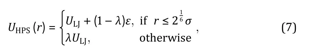
Fig. 4 Slab method to generate phase diagram using LAMMPS.A Prepare slab-like configuration. Compress the box along x- and y- dimensions to a length of approximately larger than the size of the macromolecule. Then the system was extended along zdimension. B Obtain density profile and phase diagram. Top: slice the simulation box into many pieces (or "chunks") along the z-axis, and calculate the particles in each chunk. Middle to bottom: obtain density profile along the z-axis, the derivative of which results in two absolute maximum regarded as phase boundary. Calculate the average density in both dilute ρL and dense phases ρH

Constructing a phase diagram (Step 7)

A phase diagram can provide powerful mechanism interpretations and insights for experiments. For example, it shows how variables modulate phase separation and whether phase separation can occur in physiologically relevant contexts. By merging phase diagrams of different biosystems, we can also comprehensively interpret how mutations, PTMs,different charge patterns or chemical properties influence phase separation capability.

Generating phase diagrams involves systematically varying two or more state parameters of interest, such as temperature, pressure, pH and salt concentration.For many protein-based systems, the temperature—concentration phase diagram is mainly used, especially for temperature-related proteins such as heat shock factors. The basic procedure is firstly constructing a series of systems with different protein concentrations,and then each system was simulated at a range of temperatures. Trend as a function of a third variable such as mutations can also be drawn in a phase diagram with multiple lines.

Other interpretation of the simulation results (Step 8)

Apart from phase diagrams, many other properties can also be obtained from the simulation results. MD trajectories contain all the information of the simulated system, from microscopic to macroscopic, from statics to dynamics. Thus any desired statistical properties under simulation resolution can be captured. We could calculate thermodynamic properties such as energy and pressure (McCarty et al. 2019), or further obtain dynamic information including clusters growth,droplets fusion and mean square displacement (MSD)of molecules (Alshareedah et al. 2020). Geometrical aspects can also be statistically quantified, such as the average distance of the chromocenters from the nuclear center (Falk et al. 2019) or the density distribution of IDRs along the x-axis (Bracha et al. 2019). Narrowing down to per-residue insights, one can calculate averaged configuration properties such as averaged protein valence or ratio of intermolecular interaction to intramolecular ones. Such microscopic properties are difficult to obtain experimentally but may provide significant mechanism understandings.

Approaches alternative to molecular dynamics

Another frequently used simulation algorithm is Monte Carlo (MC). Contrary to MD simulation, MC does not integrate classical equations of motion or evolve the system deterministically, but non-physical moves are performed randomly. In each step, a random move of the system is performed in the conformation space, and whether to accept the move or not depends on acceptance probability based on detailed balance,

FIELD-BASED THEORY AND SIMULATION

Compared to particle-based simulations, field-based approaches do not treat each biomolecule individually but describe their collective behaviors from a density field level. Such models enable us to characterize LLPS systems with larger scales, and despite a shortage in describing sequence-specific information, more macroscopic properties and phenomena can be examined qualitatively. Since phase separation is governed by minimization of the global free energy at equilibrium, writing down the free energy function of the system's density profile allows one to construct complete phase diagrams, study dynamic behaviors,analyze thermodynamic properties and parameter dependency in a phenomenological and predictive manner. Therefore, the critical process of field-based modeling is to determine the free energy functional suitable for the given puzzle.

A host of field-based theories has been applied or derived to describe phase separation in biosystems,many of which derived from polymer theories due to the high resemblance of associative polymers and biomacromolecules. A minimum overview of some examples and their implementations in LLPS is provided below.

Field-based theories (Step 9)

Besides the Flory—Huggins types of mixing entropy and energy, other continuous quantities contributing to the free energy can be taken into account in certain intracellular systems when necessary. For instance, Wei and coworkers (Wei et al. 2020) studied liquid—liquid phase separation in an elastic network and proposed a continuum theory with the system's free energy density which reads:

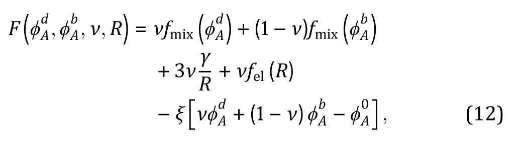
wherein the third term denotes the surface tension associated with the phase-separated droplet, the fourth term is the elastic energy related to the network elasticity, and the last term accounts for the conservation of liquid components. They found a scaling relationship between droplet size and shear modulus of the elastic network, which helps to guide fabrications of synthetic cells with desired phase properties.

To describe a biosystem with more accuracy, theories beyond mean-field approximation may also be applied.For instance, random phase approximation (RPA)theory generalized by Lin and Chan was used to describe sequence-specific phase-separation in membraneless organelles (Linet al. 2016). Field-theoretic theories developed for associative polyelectrolyte have also been used to describe biological condensation (McCarty et al.2019).

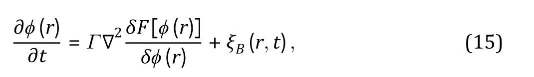
Continuum-based simulations (Steps 10-12)

PERSPECTIVES

In the protocol, we have introduced methods for unraveling phase separation mysteries in biosystems from a theoretical point of view. Different modeling scales from particle-based to field-based are described,and the global physical picture is summarized as a diagram in Fig. 5. From the atomic level, microscopic interactions and steric effects can be calculated to obtain parameters and potentials for coarse-grained simulations. Then in particle-based simulation,different coarse-grained levels can be applied to reproduce experiments and obtain various statistical properties. Going up to a larger scale, besides highefficiency simulation strategies, phenomenological theories are introduced to obtain phase diagrams and explore phase behaviors and give parameter dependencies and predictions. Finally, field-based simulations can be used to investigate dynamics in a large time scale. One should recognize that tradeoffs always exist between efficiency and accuracy. While mean-field theories such as Flory-Huggins has good approximation on phase separation behavior, particlebased frameworks will be essential to capture the nuances of sequence-dependent properties.

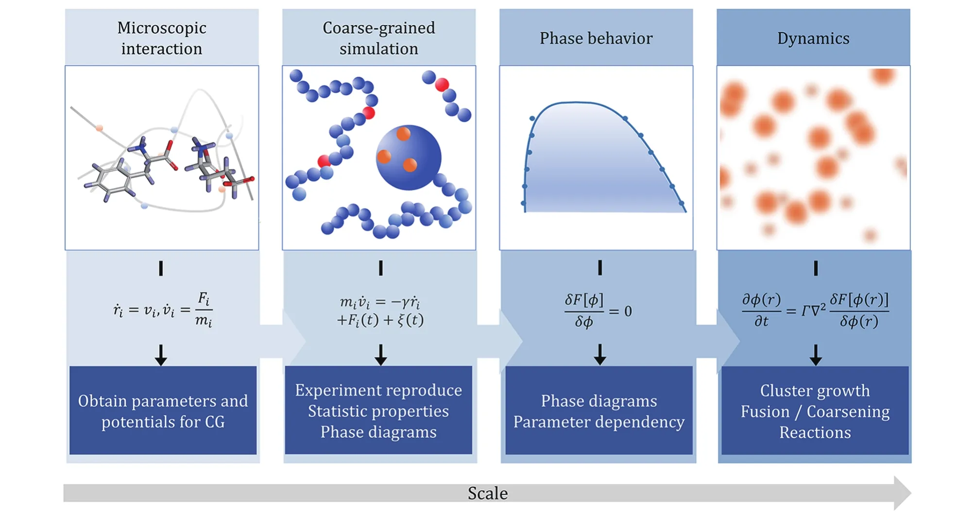
Fig. 5 Physical picture of multiscale modeling methods and their applications. From left to right are four levels of modeling method from atomistic level to coarse-grained level and then continuum field scale. The diagrams and equations represent the key methodology in each level, while the bottom boxes highlight the key words of expected results provided by the method

The given protocol will hopefully enable the readers to get started on a theoretical approach in understanding LLPS. Nevertheless, limitations and challenges still lie ahead. The main challenge is model accuracy and parameter validation. While the current coarse-grain framework can qualitatively understand and reproduce experimentations, quantitative validation and prediction are still difficult. This is due to the mesoscopic nature and complexity of biomolecular condensates, which remains challenging to date for both bottom-up mapping from atomistic computations,and top-down obtaining from experimental measurements. In this regard, the readers looking for quantitatively accurate models are encouraged to obtain parameters from experimental benchmark results, or match from results of various characterization results, such as Hi-C or NMR data(Zhang and Wolynes 2015). The second limitation is to account for nonequilibrium factors in vivo. Coarsegrained methods in this protocol are generally oversimplified with only key factors retained, which may well elucidate experiments in vitro. However, it should be noted that living-cell environments are much more complicated and are far out of equilibrium. where other nonequilibrium factors, besides aforementioned chemical reactions, may be necessary to be included to explainin vivo phase separation. For instance,intracellular species with ATP exerting forces such as filaments may be regarded as active matters,distinguished as a collection of particles converting chemical energy into mechanical work, and has arisen considerable attention in recent years (Jiang and Hou 2014; Needleman and Dogic 2017; Shelley 2016).Active particles have been found to aggregate even in the absence of attracting forces, and novel phase behaviors are found in polymer systems with active matters (Du et al. 2019a, b; Gouet al. 2021).Introducing such nonequilibrium aspects in the model may help understand some ATP-dependent processes such as the formation of stress granules or nucleoli(Brangwynneet al. 2011; Kroschwaldet al. 2015).Another important aspect of the complex environment in vivo would be the crowded cellular medium.Crowding macromolecules have proved to affect the stability and dynamics of protein phase separation significantly (André and Spruijt 2020), and packed medium molecules also introduce evident viscosity to the solution that may highly affect the dynamics of the concerned biomolecules, known as hydrodynamic interactions (Ando and Skolnick 2010). Although beyond the scope of this protocol, we do address these effects as ongoing and future research concerns.

Despite the limitations mentioned above, the current protocol is can already qualitative results for various experimentations. Simulation methods following the protocol can be used to reproduce, understand and eventually predict the effect of the mutation, PTM,change of temperature and other variables. With the appropriate coarse-grained method applied, one can efficiently perform multiple computer simulations with different condition settings, which helps to provide a global picture of parameter space and guide experimentations. In the light of ever-growing computer performance and research developments in both theory and experiments, we foresee an increasingly important role and broad application of theoretical modeling,along with growing capability in understanding physics behind intracellular phase separation.

Acknowledgements This work is supported by MOST(2018YFA0208702) and NSFC (32090040, 32090044,21833007).

Compliance with Ethical Standards

Conflict of interest Lin-ge Li and Zhonghuai Hou declare that they have no conflict of interest.

Human and animal rights and informed consent This article does not contain any studies with human or animal subjects performed by any of the authors.

Open Access This article is licensed under a Creative Commons Attribution 4.0 International License, which permits use,sharing, adaptation, distribution and reproduction in any medium or format, as long as you give appropriate credit to the original author(s) and the source, provide a link to the Creative Commons licence, and indicate if changes were made. The images or other third party material in this article are included in the article’s Creative Commons licence, unless indicated otherwise in a credit line to the material. If material is not included in the article’s Creative Commons licence and your intended use is not permitted by statutory regulation or exceeds the permitted use, you will need to obtain permission directly from the copyright holder. To view a copy of this licence, visit http://creativecommons.org/licenses/by/4.0/.