Xiao-Gu Zhong and Jian-Cheng Wang

1 Yunnan Observatories,Chinese Academy of Sciences,Kunming 650216,China;guqian29@ynao.ac.cn2 Key Laboratory for the Structure and Evolution of Celestial Objects,Chinese Academy of Sciences,Kunming 650216,China3 University of Chinese Academy of Sciences,Beijing 100049,China

Abstract We review the Seyfert 1.5 Galaxy ESO 362-G18 for exploring the origin of the soft X-ray excess.The Warm Corona and Relativistic Reflection models are two main scenarios to interpret the soft X-ray excess in active galactic nuclei at present.We use the simultaneous X-ray observation data of XMM-Newton and NuSTAR on 2016 September 24 to perform spectral analysis in two steps.First,we analyze the time-average spectra by using Warm Corona and Relativistic Reflection models.Moreover,we also explore the Hybrid model,Double Reflection model and Double Warm Corona model.We find that both the Warm Corona and Relativistic Reflection models can interpret the time-average spectra well but cannot be distinguished easily based on the time-averaged spectra fit statistics.Second,we add the rms and covariance spectra to perform the spectral analysis with time-average spectra.The result shows that the warm corona could reproduce all of these spectra well.The hot,optical thin corona and neutral distant reflection will increase their contribution with the temporal frequency,meaning that the corona responsible for X-ray continuum comes from the inner compact X-ray region and the neutral distant reflection is made of some moderate scale neutral clumps.

Key words:galaxies:active–galaxies:individual (ESO 362-G18)–galaxies:Seyfert

1.Introduction

Matter accreting into super massive black holes at the center of active galaxies is one of the most efficient mechanisms to emit electromagnetic radiation from gravitational potential energy,which covers the broad band spectrum from radio to gamma-ray.Particularly,X-ray can be used to probe the physical process of most internal regions of the accretion disk near the black hole.Generally,the X-ray continuum is considered to be from the inverse Compton scattering of the soft photons emitted by accretion disk in the hot corona.However,the details of the geometry of the corona and the radiation mechanism of disk-corona are not well understood.Especially,below 2 keV in the X-ray band,the X-ray data are above the low energy extrapolation of the best fitting continuum within 3–10 keV power law by index about 2,this is so-called soft X-ray excess.The soft X-ray excess is a major component of many active galactic nuclei (AGNs).Porquet et al.(2004) found that about 90% of the quasars in their sample exhibit significant soft X-ray excess.However,its origin has been debated over the years,and therefore,the study of soft X-ray excess is significant to discover the detail of the radiation mechanism within the innermost region of the accretion disk.Historically,the soft X-ray excess was first believed to be the hard tail of UV blackbody emission from the accretion disk (Leighly 1999).However,this explanation was ruled out because the temperature is difficult to maintain within the range of 0.1–0.2 keV for many AGNs with different masses and accretion rates.

Currently,there are some models to explain the soft X-ray excess,for example,warm corona(Czerny&Elvis 1987;Done et al.2007;Jin et al.2009;Petrucci et al.2018),relativistic reflection (Fabian et al.2002;Crummy et al.2006;Ghosh &Laha 2020;Jiang et al.2021),warm absorption(Pal et al.2016)and magnetic reconnection (Zhong &Wang 2013),in which the warm corona and relativistic reflection models are favored by many previous works.

In the warm corona case,the accretion disk photons are Comptonized by a warm (the electron temperature is below 1 keV),optical thick corona(the optical depth is between about 10 and 40),which is different from the hot(the typical value of electron temperature is 300 keV (Petrucci et al.2001)),optical thin corona (the optical depth is far less than one) that are responsible for the primary X-ray continuum.The soft X-ray excess is the high energy tail of the resulting Comptonized spectrum.Generally,the primary X-ray continuum is a cutoff power-law spectra with a typical index,Γ～1.8,in unobscured AGNs.The physical origin of the warm corona is unknown so far.The magnetic field could play a crucial role to transport the substantial amounts of energy from the disk to the warm corona vertically,then heat up the electrons in the warm corona(Merloni et al.2000;Hirose et al.2006;Begelman et al.2015).Recently,the radiative transfer computation in hydrostatic and radiative equilibrium showed that the magnetic dynamo couldheat the upper layers of the accretion flow up to a few keV for optical depths as great as ten(Gronkiewicz&Różańska 2020).García et al.(2019) put forward that the photoelectric absorption is dominant in optically thick regions by considering the coronal and photoionization equilibrium.Therefore,a forest of absorption lines are predicted in the soft X-ray spectra if the soft X-ray excess comes from the warm corona.If true,the warm corona would invalidate as an origin of the soft X-ray excess.However,Petrucci et al.(2020) and Ballantyne (2020)propose that these absorption lines could be eliminated by providing sufficient internal mechanical heating into the warm corona because the electron scattering is dominant instead of absorption opacity.

In the relativistic reflection case,a multitude of fluorescent atomic lines produced in the disk which is illuminated by the hot corona are relativistically blurred due to the proximity to the black hole.For example,the broad Fe Kα line is the prominent result of the “blurring” effect.These relativistic broadening or “blurring” lines below 2 keV will generate soft X-ray excess spontaneously and they are generally associated with the innermost stable orbit radius of disk which is determined by the black hole spin.Therefore,the relativistic reflection could be used to study the black hole spin.Another associated prominent reflection feature is the“Compton hump”which comes from the Compton down-scattering of coronal high-energy photons reprocessed in the accretion disk or distant matter (Nandra et al.1991) and achieves the peak in the reflection spectrum at about 30 keV depended on the column density as well as the geometry and inclination angle.The relativistic reflection model generally requires extreme values for the spin and hot corona compactness as well as high ionization degree.The large densities of the disk surface will enhance the soft X-ray excess (Jiang et al.2019a,2019b),which also significantly reduce the inferred iron abundances compared to typical (e.g.,with density generally equal to 1015cm-3) reflection models (e.g.,Tomsick et al.2018).

In this work,we review the Seyfert 1.5 galaxy ESO 362-G18(a.k.a.MCG 05-13-17) with redshift z=0.012 (Bennert et al.2006).Agís-González et al.(2014) (hereafter AG14) reported the black hole with a mass of (4.5±1.5)×107M⊙inferred by the virial relationship and the disk inclination of i=53°±5°obtained by using a partially ionized reflection model convolved with the KERRCONV relativistic kernel.However,Xu et al.(2021)(hereafter Xu21)report that the inclination is a lower value by using another relativistic reflection model,a sub-version of relxill (Dauser et al.2014;García et al.2014)assuming a lamppost geometry.The contradiction of the disk inclination could come from parameters degeneracy because of using different models.They propose that the black hole has a high spin～0.998 inferred by the different relativistic reflection model.But Xu21 put forward that the inner disk has a high densitywhich will enhance the soft X-ray excess.AG14 proposed that the X-ray radiation region is located within 50 gravitational radii(rg=GM/c2)by analyzing the absorption variability with 2005–2010 multi-epoch X-ray observations.Xu21 analyzed the properties of X-ray within 0.3–79 keV bands using the simultaneous X-ray observation data of XMM-Newton and NuSTAR on 2016 September 24.They find that the warm corona and the relativistic reflection model cannot be distinguished easily based on time-averaged spectra fit statistics (the same situations are also seen in,for example these recent works,García et al.2019 for Mrk509 and Liu et al.2020 for Fairall 9).However,they consider that the relativistic reflection scenario could be accepted due to its reasonable parameters,for example,the X-ray continuum index was inferred as 1.74,which is consistent with the typical value～1.8 for unobscured AGNs and without a hypothetical component such as the warm corona.They also find that the spectrum will be decoupled outside the coverage of0.5 –20 keV,and then suggest that improving theoretical models and future observations covering wider energy bands with high resolution are essential for exploring the nature of the soft X-ray excess.

The paper is organized as follows.In Section 2,we present the observational data.In Section 3,we analyze the time properties.In Section 4,we perform the spectral analysis.Finally,we discuss our results and conclude in Section 5.

2.Observation Data

We use the simultaneous X-ray observation data of NuSTAR(Harrison et al.2013) and XMM-Newton (Jansen et al.2001)on 2016 September 24 to perform the spectral analysis for ESO 362-G18.The observation ID are 60201046002 for NuSTAR with 100 ks net exposure and 0790810101 for XMM-Newton with 120 ks net exposure.The observation information that we used in the paper is shown in Table 1.

2.1.NuSTAR Data Reduction

The reduction of the NuSTAR data is conducted following the standard procedures using the NuSTAR Data Analysis Software (NUSTARDAS v.2.0.0).We use nupipeline and the 20210427 version of NuSTAR CALDB to produce clean event files.We use the “nucalcsaa” module to calculate South Atlantic Anomaly (SAA) and set the input parameter“saacalc=2,” “saamode=STRICT” to choose the strict mode.The circular source region is a radius of 60″.In order to avoid the background dominance,we select eight circular regions with repeating attempts to extract the background spectra .Figure 1 shows the NuSTAR FPMA event image for extracting the source and background spectrum,and the total area of background is larger than the source.We then utilize the task package nuproducts to extract the source and background light curves (shown in the top two panels of Figure 2) and spectra.The spectra are grouped to at least 30 counts in each bin in order to have high signal-to-noise ratio.

2.2.XMM-Newton Data Reduction

For XMM-Newton,we only use EPIC-pn data in 0.3–10 keV to do the spectral analysis.The raw data are processed from Observation Data Files following standard procedures based on the Science Analysis System (SAS v16.1.0) and the latest calibration files.The spectra and light curve are extracted using tool evselect with default pattern selected.We extract the source spectra and light curve from a circular region with the radius of 35″ centered on the source.The background spectra are taken from a circular region with the same size near the source but excluding source photons.rmfgen and arfgen are used to produce response matrices.Source spectra are rebinned by grppha with a minimum of 30 counts per bin.epiclccorr is used to correct the light curve (shown in the bottom panel of Figure 2).We test the pile-up for these data by using epatplot and find that the pile-up is not important to ESO 362-G18.

3.Time Analysis

We analyze the variability properties by only using the XMM-Newton observation data because NuSTAR is a nearearth satellite with the altitude～650 km×610 km,its data is discontinuous due to the occlusion by Earth every 5 ks(seen in the top two panels of Figure 2) to distort the power spectral density (PSD).We calculate PSD by choosing a bin time of 400 s to ensure that there are no zero-count bins contained in the light curves (Jin et al.2021).The PSD can be calculated from the periodogram(Vaughan&Nowak 1997;Nowak et al.1999),

where Xnis the discrete Fourier transform (DFT),

at each Fourier frequency,fn=n/(NΔt),where n=1,2,3...N/2,N is the number of tine bins of width Δt.The maximum frequency is the Nyquist frequency,xkis the kth value of the light curve.The asterisk denotes complex conjugation.Then,the normalized PSD could be calculated as follows:

where 〈x〉 is the average count rate in the light curve.We then calculate the time lag between the soft band 0.3–1 keV and hard band 1–4 keV by estimating the Fourier cross spectrum between the two energy band light curves x(t) and y(t) with DFTs,Xnand Yn(Zoghbi et al.2010;Kara et al.2013),as follows:

where CXY,nis the Fourier cross spectrum.The time lag between the two energy bands is estimated by

We find that the hard band lags behind the soft band,called hard-lag,at lower frequencies.However,the soft band lags behind the hard band,called soft-lag,at higher frequency except[1.3–5.4]×10-4Hz,but this lag could be unreal due to its low signal-noise ratio.The soft-lag at[0.5–1.3]×10-4Hz is distinct,which is consistent with the work of AG14 (seen Figure 9 in AG14).It is noted that the lag is significant when two energy bands have prominent correlation.Therefore,we test the coherence of two energy bands,γ2,defined as(Nowak et al.1999;Zoghbi et al.2010):

where the bar above parameters means the average value with the frequency bin.The coherence between the two energy bands is shown in Figure 4,we select lager frequency bin at the lowest frequency bin to ensure statistical efficiency and we find that there are good correlations at low frequency bands,especially γ2～1 at the lowest frequency bin,which implies a small error bar.In contrast,the higher frequency has a bad correlation,especially γ2～0 at the highest frequency bin,which also implies a small error bar.

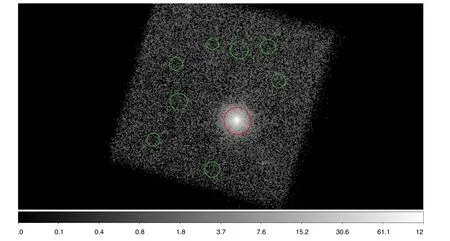
Figure 1.NuSTAR FPMA event image of observation ID 60201046002(ESO 362-G18)displayed in ds9.The source spectrum is extracted from the red circle region and the background spectrum is extracted from these eight green circles shown in ds9.

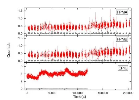
Figure 2.The light curve of NuSTAR FPMA,FPMB and XMM-Newton EPIC from top to bottom panel.The red and gray data represent source and background light curves,respectively.

Figure 3.The frequency-dependent lags between the hard band at 1–4 keV and the soft band at 0.3–1 keV.

Figure 4.The frequency-dependent coherence between the hard band at 1–4 keV and the soft band at 0.3–1 keV.

In order to analyze the energy-dependent variability in the general,we focus on three frequencies,the low frequency([1–2]×10-5Hz),the middle frequency([0.5–1.3]×10-4Hz)and the high frequency ([0.5–1.3]×10-3Hz).The energy bin we adopt is 100 eV if we do not state otherwise.Figure 5 shows the energy-dependent coherence of low,middle and high frequencies for each energy bin,the reference energy band we selected is the whole energy band of XMM-Newton data,0.3–10 keV,but excluding the interested energy bin themselves.It displays that the correlation decreases from low to high frequency and from low to high energy band in low and middle frequencies.The high frequency has a poor correlation.

Figure 6 shows more details about the time lags of low,middle and high frequencies for each energy bin,the reference energy band is also the whole energy band of XMM-Newton data,0.3–10 keV,but excluding the interested energy bin themselves to reduce self-correlation.It displays a clear hardlag at the low frequency.It is indicated that the variability is propagated from soft to hard energy band in a larger scale.There are no clear lags below 3 keV in middle frequency,but it has some leading at 3–5 keV and then has some lag at a high energy,about 8–10 keV,which may show the reverberation characteristics because 3–5 keV energy band represents the X-ray continuum radiated from hot corona to illuminate the disk,and the lag at 8–10 keV could be a tail of “Compton hump”that is a reflection feature.The high frequency does not show any significant lags.

The root mean square (rms) describes the degree of the variability and is classified into fractional rms and absolute rms(hereafter we use the capital,rms,represents the absolute rms),where fractional rms is defined as (Vaughan et al.2003):

The covariance is the cross-spectral counterpart of the rms,which measures the rms amplitude of variability as a detailed function of energy (Wilkinson &Uttley 2009):

whereand PY,noiseare the reference band and noise of PSD,respectively,which are adopted at the whole energy band from 0.3 to 10 keV and removed the light curve of the interested energy bin for each channel to avoid the self-correlation by themselves just like mentioned above.Figures 8 and 9 show the energy-dependent rms and covariance of low,middle and high frequencies for each energy bin.The covariance displays the same shape as the rms.However,the signal-to-noise of the covariance is better than that of rms,since the reference band light curve is effectively used as a “matched filter” to pick out the correlated variations in each energy bin.It is noted that we adopt wider energy bins above 2.3 keV,which are larger than100 eV stating above,so the rms and covariance spectra can be extended to 10 keV and avoid the zero-count bin contained in the light curves in both of Figures 8 and 9.However,based on the definition of the rms and covariance mentioned above,both of them depend on the average count rate of the light curve,〈x〉,which relies on the scale of energy bin.Therefore,the rms and covariance have the deviation above 2.3 keV because the inhomogeneous energy bins are adopted to avoid the zero-count contained in the light curves.If the time bin we adopt is larger than 400 s,it helps to extend the energy band range and ensure the homogeneous energy bins for the rms and covariance spectra,but it loses the information of high frequency.In order to cover the whole energy band and ensure the homogeneous energy bins for the rms and covariance spectra,the scale of energy bin could be adopted as the energy bin of the highest energy band at about 8–10 keV,which will ensure that each energy bin does not include zero-count because the count rate of the highest energy band is more less than lower energy band.But it will lose the detailed information of the soft energy band (0.3–1 keV) because one energy bin could cover the soft energy band.We will analyze the rms and covariance in detail in following section of spectra analysis.

Figure 5.The energy-dependent coherence of low,middle and high frequencies for each energy bin from left to right panel.The reference energy band is the whole energy band of XMM-Newton data,0.3–10 keV,but excluding the interested energy bin themselves to reduce self-correlation.

Figure 6.The energy-dependent lags of low,middle and high frequencies for each energy bin from left to right panel.The reference energy band is the whole energy band of XMM-Newton data,0.3–10 keV,but excluding the interested energy bin themselves to reduce self-correlation.

Figure 7.The energy-dependent fractional rms of low,middle and high frequencies for each energy bin from left to right panel.

Figure 8.The energy-dependent rms of low,middle and high frequencies for each energy bin from left to right panel.

Figure 9.The energy-dependent covariance of low,middle and high frequencies for each energy bin from left to right panel.

4.Spectral Analysis

We use the XSPEC software (v12.11.1) (Arnaud 1996) to analyze the energy spectrum of ESO 362-G18.The summary of the models used in the paper is shown in Table 2.The first two models are the most favored competing models,Warm Corona and Relativistic Reflection.We also explore the Hybrid model which includes the warm corona and relativistic reflection components,Double Reflection model which includes two relativistic reflection components and the Double Warm corona model which includes two warm corona components.The Crossnormalization,constant,is fixed as one for the XMM-Newton data and set free for NuSTAR FPMA/B.We use two absorption model,tbabs (Wilms et al.2000),to describe the Galactic absorption with setting the Galactic absorption hydrogen column density at 1.75×1020cm-2(Kalberla et al.2005) during the spectral fitting with abundance set to wilms (Wilms et al.2000)with vern cross-section(Verner et al.1996),and the version with redshift,ztbabs,to describe the neutral absorption component for the host of galaxy of ESO 362-G18 with fixing redshift at z=0.012 and a free absorption hydrogen column density.zxipcf(Reeves et al.2008) is used to fit the warm absorber proposed by AG14 and Xu21.We use the thermal Comptonization model,nthcomp(Życki et al.1999),to fit the X-ray continuum radiated from hot corona.The seed photon temperature of disk,kTdisk,is fixed at 3 eV.The physical torus model,borus12 (Baloković et al.2019),be used to fit the distant reflection as Xu21 did and we fix the cosine of the torus inclination angleor=37°.The photon index,Γ,and electron temperature,kTe,are linked with the hot corona radiation,nthcomp.The Spectral Analysis has two steps as follows:The first step is fitting the time-average spectra simultaneously by using above models.The second step is not only the same fitting recipes like as the first step,but also add the rms and covariance spectrum into the fit simultaneously with the time-average spectra.The rms and covariance data are just adopted from 0.3 to 2.3 keV due to avoid the non-uniform energy bin influenced by the zero-count contained in the light curves,which will bring the deviation to the result of spectral analysis.We will plot the fitting results of the time-average spectra and the rms and covariance spectrum onthe same figure for the second step with different units,in which the photon flux unit,photons cm-2s-1keV-1,is used for the time-average spectra and the count rate unit,counts s-1,is used for the rms and covariance spectrum.The two units actually differ by one normalized factor because the response file could be assumed a unit diagonal matrix for the rms and covariance spectrum,and the uniform energy bin is adopted.

Table 2 The Summary of the Model Used in the Paper

Table 3 Fitting Results of Warm Corona Model for Step 1 and 2

4.1.Warm Corona Model

We add a second thermal Comptonization component,nthcomp,to fit the soft X-ray excess.The seed photon temperature of the warm corona component also is also fixed at 3 eV.The fitting results are shown in Table 3 and Figure 10.

Figure 10.The fitting results of the Warm Corona model for step 1 and 2 shown in left and right panels,respectively.Black,red and green data points are the timeaverage spectrum of XMM-Newton,NuSTAR FPMA,and FPMB data,respectively.Blue,cyan and magenta data points are the covariance spectrum of low,middle and high frequencies,respectively.The corresponding color lines are the best fitting results.Orange,dark yellow and olive lines represent the radiation of hot corona,warm corona and the distant material reflection,respectively.The dashed,dashed–dotted and dotted lines represent the fitting results of covariance spectrum of low,middle and high frequencies with each model component which is as same color as the corresponding solid lines.The photon flux unit,photons cm-2 s-1 keV-1,is used for the time-average spectra and the count rate unit,counts s-1,is used for the covariance spectrum in the right panel.The bottom panel is the data-to-model ratio.

4.1.1.The First Step

The Chi-square values/d.o.f of fitting result is 1061/959(reduced χ2=1.11).The hydrogen column density of the host galaxy absorption is less than 1.09×1020cm-2.The ionization degree,logξof warm absorber,zxipcf,is very low,which means that the radiation is absorbed by neutral material.The column density of warm absorber,NHis order of 1021cm-2,which is an order of magnitude larger than that of Xu21,but consistent with the result of AG14 who also used the zxipcf to model the warm absorber,it could be using different warm absorption model.The X-ray continuum index,Γ=1.63±0.02,and the electron temperature of hot corona,kTe=20.66±4.27 keV,are consistent with the result of Xu21,however,it is not reasonable because the optical depth is optical thick.The photon index of warm corona is 1.81±0.27 instead of the fixed value of 2.5 adopted by Xu21.The electron temperature of warm corona is 0.16±0.01 keV which is consistent with the result of Xu21.But the corresponding optical depth of the warm corona is about 50,which is larger than the prediction of Ursini et al.(2020) (10～40).

4.1.2.The Second Step

The Chi-square values/d.o.f of fitting result is 1171/977(reduced χ2=1.19),which is worse than that of the first step.The hydrogen column density of the host galaxy absorption is obtained about an order of 1020cm-2as same as the Galactic absorption.In the right panel of Figure 10,we add the covariance spectrum of low,middle and high frequencies into plot for comparison with the time-average spectrum.Figure 11 shows the detailed fitting result of variability spectrum (rms and covariance spectrum)and the deviation mainly comes from the variability spectrum fitting,which displays that the X-ray continuum radiated from hot corona is the main contributor,but the reflection of distant material,borus12,increases the contribution at high frequency.The Warm model cannot interpret the residual error shown in the right panel of Figure 11.

4.2.Reflection Model

Like Xu21,we implement the relativistic reflection with variable disk density,relxilllpd to be as the soft X-ray excess component with the lamp post geometry (Dauser et al.2014;García et al.2014,2016).We set the disk inclination to be free and the inner/outer disk radius to be the default values.The incident spectral index of the relativistic reflection is linked with the X-ray continuum.We fix the electron temperature of hot corona,kTe=300 keV.The fitting results are shown in Table 4 and Figure 12.

Figure 11.The fitting results of the rms and covariance spectrum shown in the left panel by using the Warm Corona model.The black,red and blue lines represent the fitting results,the Comptonization radiation of hot corona and the reflection of distant material,respectively.The data-to-model ratio is shown in the right panel.

4.2.1.The First Step

The Chi-square values/d.o.f of the fitting result is 1073/956(reduced χ2=1.12),which cannot be distinguished easily compared with the Warm corona model in the first step.The hydrogen column density of the host galaxy absorption has an upper limit value,NH(1020cm-2)＜0.73.The X-ray continuum index,Γ=1.68±0.05,is less than the typical index,Γ～1.8 but reasonable because it is according with the physical property of optical thin for hot corona with the electron temperature of 300 keV.The height of corona is h=2.53±1.49rg,which means that the hot corona is compact just as the prediction of microlensing (e.g.,Dai et al.2010;Mosquera et al.2013).The fitting result shows the black hole has a high spin,a=0.998.The disk inclination is less than 67°.59.The ionization degree of disk is obtained a higher value than that obtained by Xu21.The iron abundances cannot be constrained in the fitting and is pegged atand the disk density is obtained atHowever,the iron abundances and the disk density could be degenerated(Tomsick et al.2018).

4.2.2.The Second Step

The Chi-square values/d.o.f of the fitting result is 1268/974(reduced χ2=1.30),which is worse than that of the first step and the Warm corona model in the second step.The hydrogen column density of the host galaxy absorption is obtained a moderate value NH(1020cm-2)=1.07±0.34.The X-ray continuum index,Γ=1.68±0.04,which is less than the typical index.The height of corona is h=2.58±0.88rgconsistent with the first step.The black hole spin also has a high value.The disk inclination is obtained an upper value,＜34°.09.In the right panel of Figure 12,we add the covariance spectrum of low,middle and high frequencies into plot for comparison with the time-average spectrum.Figure 13 shows the detailed fitting result of the variability spectrum.The X-ray continuum radiated from hot corona and the reflection of distant material are the main contributor,but still cannot interpret the residual error.

4.3.Hybrid Model

The Hybrid model considers that the soft X-ray excess comes from both of warm corona and relativistic reflection.We adopt the standard relativistic reflection model,relxillcp,which assume the incident radiation is a Comptonization continuum.Like the set of Warm Corona model,we set the seed photon temperature to be 3 eV for the second nthcomp component.We set the index of emissivity to be q1=q2=3,the inner radius of the disk is 50rgand the outer of disk is the default value,assuming that the relativistic reflection component is out of the warm corona,so the relativistic effects could be weak.The electron temperature is also fixed at 300 keV as the Reflection model,the disk inclination is set to be free.The photon index of the relativistic reflection is linked with the hot corona.The fitting results are shown in Table 5 and Figure 14.

Table 4 Fitting Results of Reflection Model for Step 1 and 2

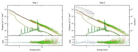
Figure 12.The fitting results of the Reflection model for step 1 and 2 shown in the left and right panels,respectively.Black,red and green data points are the timeaverage spectra of XMM-Newton,NuSTAR FPMA,and FPMB data,respectively.Blue,cyan and magenta data points are the covariance spectrum of low,middle and high frequencies,respectively.The corresponding color lines are the best fitting results.Orange,dark yellow and olive lines represent the radiation of hot corona,relativistic reflection and the distant material reflection,respectively.The dashed,dashed–dotted and dotted lines represent the fitting results of covariance spectrum of low,middle and high frequencies with each model component which is as same color as the corresponding solid lines.The photon flux unit,photons cm-2 s-1 keV-1,is used for the time-average spectra and the count rate unit,counts s-1,is used for the covariance spectrum in the right panel.The bottom panel is the data-to-model ratio.

Figure 13.The fitting result of the rms and covariance spectrum shown in the left panel by using the Reflection model.The black,red and blue lines represent the fitting result,the Comptonization radiation of hot corona and the reflection of distant material,respectively.The data-to-model ratio is shown in the right panel.

Figure 14.The fitting results of the Hybrid model for step 1 and 2 shown in left and right panel,respectively.Black,red and green data points are the time-average spectra of XMM-Newton,NuSTAR FPMA,and FPMB data,respectively.Blue,cyan and magenta data points are the covariance spectrum of low,middle and high frequencies,respectively.The corresponding color lines are the best fitting results.Orange,dark yellow,olive and purple lines represent the radiation of hot corona,warm corona,the reflection of distant material and the relativistic reflection,respectively.The dashed,dashed–dotted and dotted lines represent the fitting results of covariance spectrum of low,middle and high frequencies with each model component which is as same color as the corresponding solid lines.The photon flux unit,photons cm-2 s-1 keV-1,is used for the time-average spectra and the count rate unit,counts s-1,is used for the covariance spectrum in the right panel.The bottom panel is the data-to-model ratio.

4.3.1.The First Step

The Chi-square values/d.o.f of the fitting result is 1031/955(reduced χ2=1.07),which obtains the best fitting compared with the other four models in the first step.The hydrogen column density of the host galaxy absorption has an upper limit value,NH(1020cm-2)＜0.48.The X-ray continuum index,Γ=1.75±0.02,is consistent with the typical index.The photon index and electron temperature of warm corona are 2.08±0.10 and 0.19±0.03 keV,where the optical depth of the warm corona is about 40,consistent with the prediction of Ursini et al.(2020).The black hole spin also get a high value,a=0.97.The ionization degree of disk takes a moderate value,The iron abundances has a sub-solar value AFe=0.49±0.11 consistent with the result of Xu21.

4.3.2.The Second Step

The Chi-square values/d.o.f of the fitting result is 1144/967(reduced χ2=1.18),which is worse than that of the first step.The hydrogen column density of the host galaxy absorption is obtained about an order of 1020cm-2as same as the Galactic absorption.Other parameters obtained by the fitting result are consistent with those of the first step.In the right panel of Figure 14,we add the covariance spectrum of low,middle and high frequencies into plot for comparison with the time-average spectrum.The deviation mainly comes from the variability spectrum fitting (Figure 15),which displays that the X-ray continuum radiated from hot corona is the main contributor,the reflection of distant material,borus12,increases the contribution at high frequency.But it can still also not interpret the residual error in the right panel of Figure 15.

4.4.Double Reflection Model

Double relativistic reflection components are considered to be the mechanism of the soft X-ray excess and other reflection features.We adopt the first reflection model with lamp post geometry and variable disk density,relxilllpd,which describes the reflection process of inner compact region and the second reflection model,relxillcp,with coronal geometry that assumes a density of 1015cm-2,which is different from the first reflection component and outside of inner compact region of black hole.Therefore,we set the index of emissivity to be q1=q2=3,the inner radius of the disk is 50rgand the outer of disk is the default value.We still fix the electron temperature at 300 keV.The photon index of two reflection components is linked to the hot corona.The iron abundances and disk inclination are linked with each other.The fitting results are shown in Table 6 and Figure 16.

Table 5 Fitting Results of Hybrid Model for Step 1 and 2

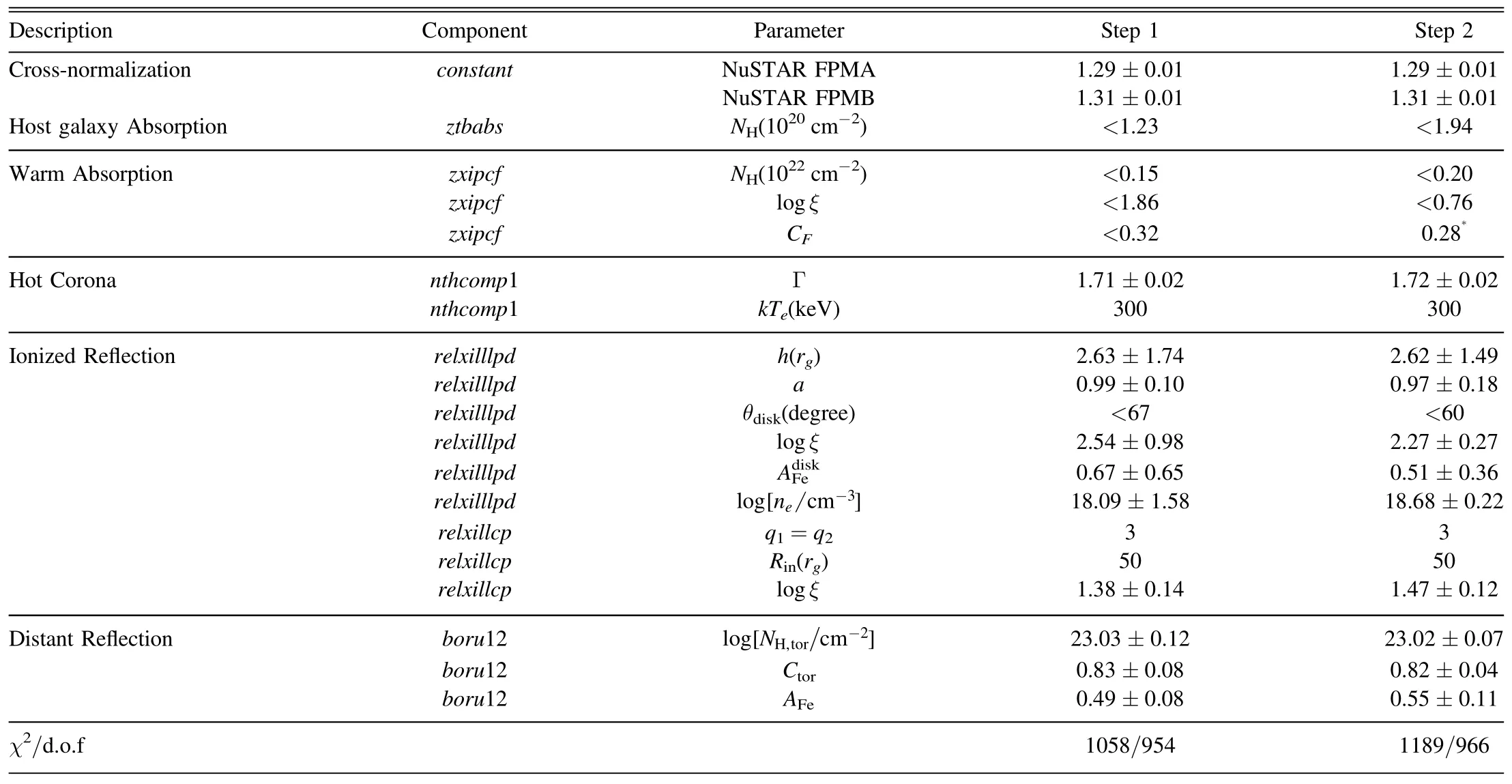
Table 6 Fitting Results of Double Reflection Model for Step 1 and 2

Figure 15.The fitting results of the rms and covariance spectrum shown in the left panel by using the Hybrid model.The black,red and blue lines represent the fitting results,the Comptonization radiation of hot corona and the reflection of distant material,respectively.The data-to-model ratio is shown in the right panel.

4.4.1.The First Step

The Chi-square values/d.o.f of the fitting result is 1058/954 (reduced χ2=1.10),which cannot be distinguished easily compared with the Warm corona and Reflection model in the first step.The hydrogen column density of the host galaxy absorption has an upper limit value,NH(1020cm-2)＜1.23.The photon index of hot corona is Γ=1.71±0.02 which is consistent with the typical value.The black hole spin also has a high value about 0.99.The ionization degree has a high value logξ=2.54 ± 0.98for the first reflection and a moderate value,logξ=1.38 ±0.14 for the second reflection.The disk iron abundance is less than one but with a high error.

4.4.2.The Second Step

The Chi-square values/d.o.f of the fitting result is 1189/966(reduced χ2=1.23),which is worse than that of the first step.In the right panel of Figure 16,we add the covariance spectrum of low,middle and high frequencies into plot for comparison with the time-average spectrum.However,the parameters obtained by the fitting result are consistent with those of the first step.The deviation mainly comes from the rms and covariance spectrum fitting (Figure 17).The two relativistic reflection components do not contribute to the variability spectrum.The radiation of hot corona can also not interpret the variability spectrum although it has a high contribution at the low frequency.

Figure 16.The fitting results of the Double Reflection model for step 1 and 2 shown in the left and right panels,respectively.Black,red and green data points are the time-average spectrum of XMM-Newton,NuSTAR FPMA,and FPMB data,respectively.Blue,cyan and magenta data points are the covariance spectrum of low,middle and high frequencies,respectively.The corresponding color lines are the best fitting results.Orange,dark yellow,olive and purple lines represent the radiation of hot corona,the first reflection,relxilllpd,the second reflection,relxillcp,and the reflection of distant material.The dashed,dashed–dotted and dotted lines represent the fitting results of covariance spectrum of low,middle and high frequencies with each model component which is as same color as the corresponding solid lines.The photon flux unit,photons cm-2 s-1 keV-1,is used for the time-average spectra and the count rate unit,counts s-1,is used for the covariance spectrum in the right panel.The bottom panel is the data-to-model ratio.

Figure 17.The fitting results of the rms and covariance spectrum shown in the left panel by using the Double Reflection model.The black,red and cyan lines represent the fitting results,the Comptonization radiation of hot corona and the reflection of distant material,respectively.The data-to-model ratio is shown in the right panel.

4.5.Double Warm Corona Model

The Double Warm Corona model is made of two warm corona components,which was used to interpret the origin soft X-ray excess and X-ray Quasi-Periodic Oscillation for the famous Seyfert 1 galaxy,RE J1034+396 in the work of Jin et al.(2021).We also explore the model for ESO 362-G18.The seed photon temperature of the two warm coronas are fixed at 3 eV.The electron temperature of the hot corona is fixed at 300 keV.The fitting results are shown in Table 7 and Figure 18.

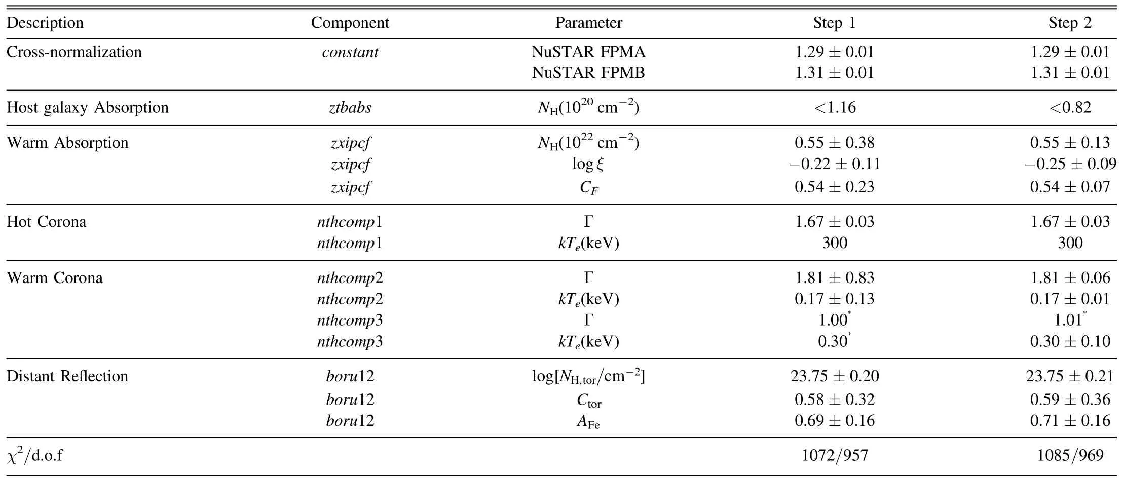
Table 7 Fitting Results of Double Warm Corona Model for Step 1 and 2

4.5.1.The First Step

The Chi-square values/d.o.f of the fitting result is 1072/957(reduced χ2=1.12).The hydrogen column density of the host galaxy absorption has an upper limit value,NH(1020cm-2)＜1.16.The photon index of hot corona has a low value compared with the typical value,Γ=1.67±0.03.The first warm corona has a soft spectrum of Γ=1.81,and the electron temperature is 0.17 keV,it corresponds the optical depth to be about 53.However,the second warm corona cannot constrain the spectrum index and the electron temperature,and it is a reasonable result because the second warm corona is weak compared with other components in the first step (left panel of Figure 18) and the data cannot constrain the component effectively.

Figure 18.The fitting results of the Double Warm Corona model for step 1 and 2 shown in the left and right panels,respectively.Black,red and green data points are the time-average spectrum of XMM-Newton,NuSTAR FPMA,and FPMB data,respectively.Blue,cyan and magenta data points are the covariance spectrum of low,middle and high frequency,respectively.The corresponding color lines are the best fitting results.Orange,dark yellow,olive and purple lines represent the radiation of hot corona,the first warm corona,the reflection of distant material and the second warm corona,respectively.The dashed,dashed–dotted and dotted lines represent the fitting results of covariance spectrum of low,middle and high frequencies with each model component which is as same color as the corresponding solid lines.The photon flux unit,photons cm-2 s-1 keV-1,is used for the time-average spectra and the count rate unit,counts s-1,is used for the covariance spectrum in the right panel.The bottom panel is the data-to-model ratio.

4.5.2.The Second Step

The Chi-square values/d.o.f of the fitting result is 1085/969(reduced χ2=1.12),which is the best fitting result of all of the second step mentioned above and means that the double warm corona model could interpret the variability spectrum well(Figure 19).We find that the second warm is dominant at low frequency,the hot corona and the distant reflection increase their contribution at high frequency.The photon index of hot corona,Γ=1.67±0.03,is consistent with that of the first step.The first warm corona’s photon index is 1.81±0.06 and the electron temperature is 0.17 keV,which corresponds the optical depth to be about 53.The second warm corona’s photon index is pegged a very low value which corresponds the optical depth to be a very high value.

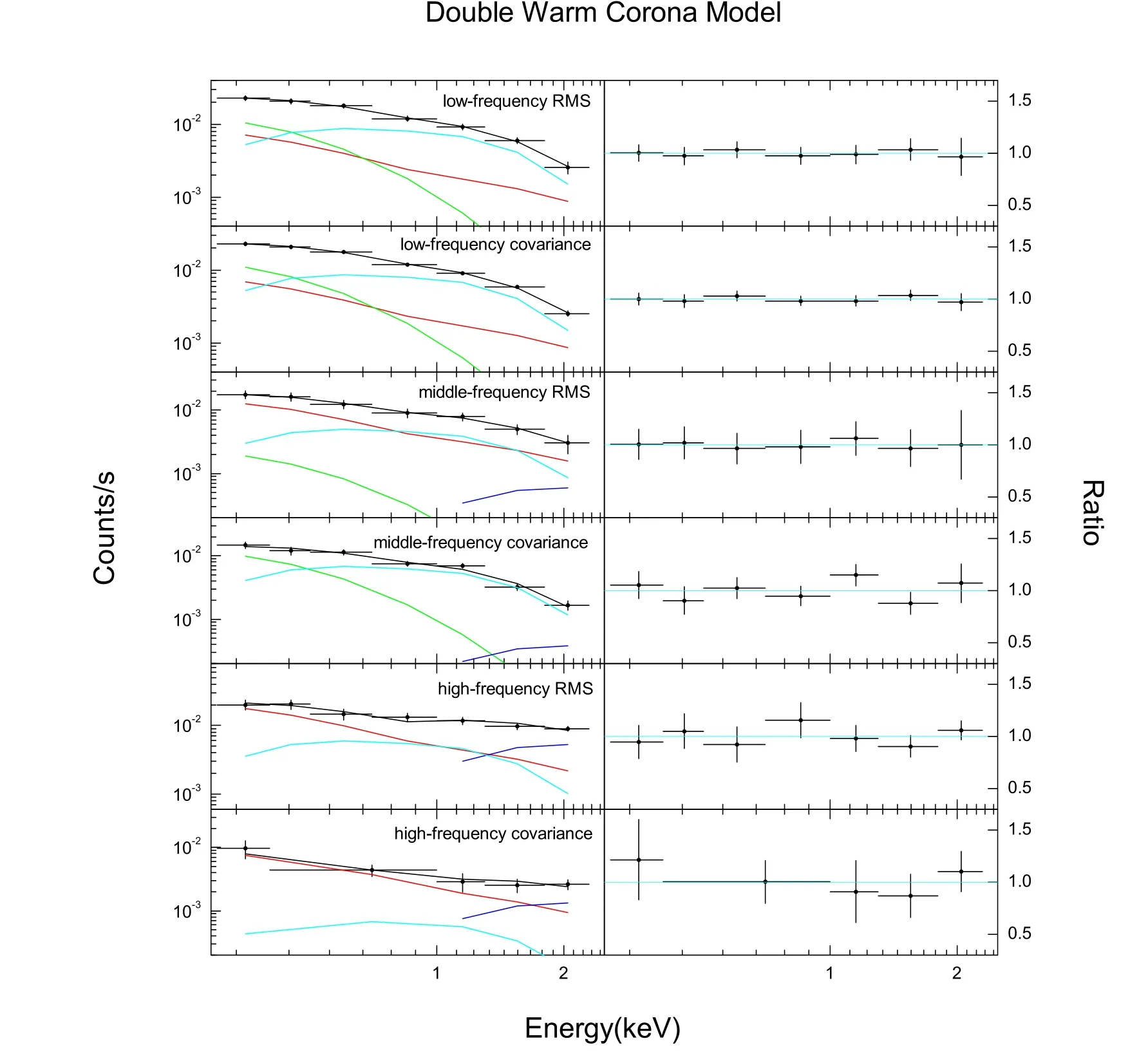
Figure 19.The fitting results of the the rms and covariance spectrum shown in the left panel by using the Double Warm Corona model.The black,red,green,cyan and blue lines represent the fitting results,the Comptonization radiation of hot corona,the first warm corona,the second warm corona,and the reflection of distant material,respectively.The data-to-model ratio is shown in the right panel.

4.5.3.Constrain the Optical Depth

Through the above analysis,the double warm corona model could reproduct both of the time-average spectrum and the variability spectrum.However,the fitting result shows that the optical depth of the second warm corona are too high to be impenetrable based on previous work.The thermally Comptonized continuum model,nthcomp,has two main free parameters such as the photon index,Γ,and the electron temperature,kTe.The optical depth is inferred from two parameters by the formula as follows (Zdziarski et al.1996):

where τ is the optical depth,meis the electron mass,mec2is 511 keV,and Γ is the photon index.Therefore,the optical depth could be evaluated from the above formula easily.However,the optical depth is not constrained easily in fitting process by using the nthcomp model in XSPEC.In order to solve the problem,we adopt the Comptonization of soft photons in a hot plasma model,comptt,to fit the soft X-ray excess and replace nthcomp.comptt also has two main freeparameters such as the electron temperature,kTeand optical depth,τ.So,we can constrain the optical depth directly in the fitting process.The fitting results are shown in Table 8 and Figure 20 for the second step.Chi-square values/d.o.f of the fitting result is 1081/969 (reduced χ2=1.11).The photon index has a low value,Γ=1.66±0.03 compared with the typical value.The optical depths of two warm coronas are constrained well due to fitting with the variability spectrum,which is consistent with the prediction of Ursini et al.(2020).The second warm corona component contributes for the fitting statistics aswhich implies the second warm corona component is significant.Figure 21 shows the detailed fitting result of the variability spectrum,which displays the second warm corona component to be the main generation mechanism,and the hot corona and distant reflection dominant the radiation gradually at the high frequency.

Figure 20.The fitting results of the double warm corona model by using comptt for step 2 only.Black,red and green data points are the XMM-Newton,NuSTAR FPMA,and FPMB data,respectively.Blue,cyan and magenta data points are the covariance spectrum of low,middle and high frequencies,respectively.The corresponding color lines are the best fitting results.Orange,dark yellow,purple and olive lines represent the radiation of hot corona,the first warm corona,the second warm corona and the reflection of distant material.The dashed,dashed–dotted and dotted lines represent the fitting results of covariance spectrum of low,middle and high frequency with each model component which is as same color as the corresponding solid lines.The photon flux unit,photons cm-2 s-1 keV-1,is used for the time-average spectra and the count rate unit,counts s-1,is used for the covariance spectrum.The bottom panel is the data-to-model ratio.

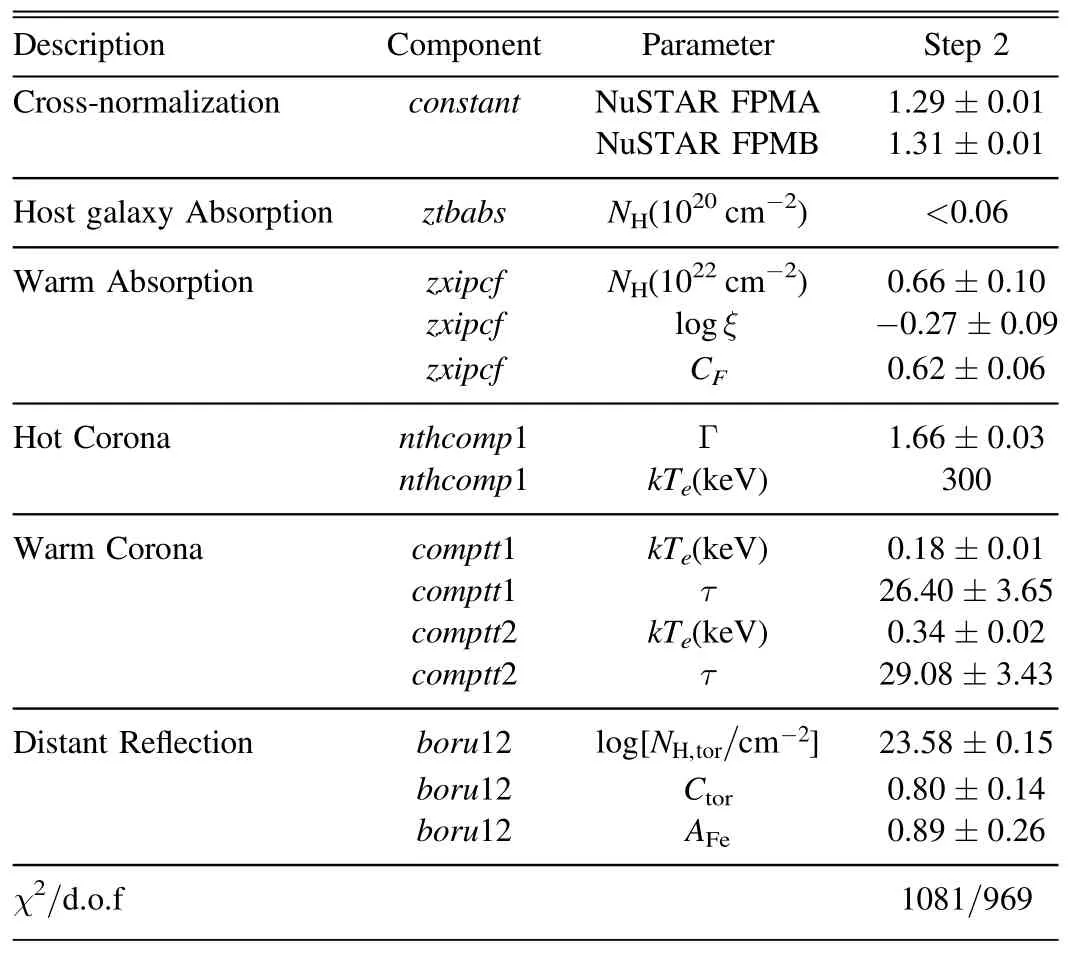
Table 8 Fitting Results of Double Warm Corona Model Only for Step 2 by Using comptt

5.Discussion and Conclusions

5.1.Comparing with Xu21

ESO 362-G18 had been explored in detail by Xu21 using warm corona and relativistic reflection models,and has the same data as we adopt.We use the same model of Xu21 to review the source by employing the XSPEC software with our data set.We fix all of parameters obtained by Xu21 and the Chi-square values/d.o.f are 1317/1032 for the warm corona model(Model A from Table 2 of Xu21),1712.86/1030 for the relativistic reflection model (Model B from Table 2 of Xu21)and 1183/1030 for the hybrid model(Model C from the Table 2 of Xu21).Even so,we also obtain a compact hot corona(h～3rg) and a rapidly spinning black hole consistent with Xu21.However,the relativistic reflection cannot interpret the variability spectrum well in our work.Therefore,the spectral analysis combining with average-time spectrum and variability spectrum could help to decouple the different components which cannot be distinguished easily based on only time-averaged spectra fit statistics.

In part 3 of Xu21,they test the neutral reflection model,xillver(García&Kallman 2010),and find the Fe K emission is overpredicted.So they instead use the borus12 model as we used in this paper.We also test the neutral reflection model replaced the borus12 model in the Double Warm Corona model.Figure 22 shows the fitting result of the scenario in the second step and the first warm corona component has little contribution for the spectrum.We find that the neutral reflection model cannot interpret the covariance spectrum in the high frequency,which implies the neutral reflection does not include the cold disk reflection radiation in the soft energy band in ESO 362-G18.

Figure 21.The fitting results of the rms and covariance spectrum shown in the left panel by using the double warm corona model which adopt the comptt model.The black,red,green,cyan and blue lines represent the fitting results,the Comptonization radiation of hot corona,the first warm corona,the second warm corona,and the reflection of distant material,respectively.The data-to-model ratio is shown in the right panel.

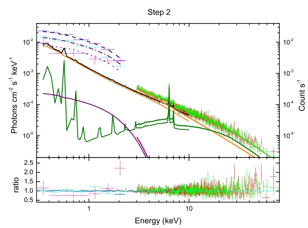
Figure 22.The fitting results of the double warm corona model and replace borus12 with the neutral reflection model,xillver for step 2 only.Black,red and green data points are the XMM-Newton,NuSTAR FPMA,and FPMB data,respectively.Blue,cyan and magenta data points are the covariance spectrum of low,middle and high frequencies,respectively.The corresponding color lines are the best fitting results.Orange,purple and olive lines represent the radiation of hot corona,the second warm corona and the neutral reflection,respectively.The first warm corona component has little contribution for the spectrum.The dashed,dashed–dotted and dotted lines represent the fitting results of covariance spectrum of low,middle and high frequencies with each model component which is as same color as the corresponding solid lines.The photon flux unit,photons cm-2 s-1 keV-1,is used for the time-average spectra and the count rate unit,counts s-1,is used for the covariance spectrum.The bottom panel is the data-to-model ratio.

Figure 23.The energy-dependent covariance of low,middle and high frequencies compared with time-average spectra for each energy bin from left to right panel.The black and red data points are the time-average spectrum and covariance data,respectively.The blue solid line represents the continuum radiation of hot corona.

5.2.The Photon Index of Hot Corona Interpretation

From spectral analysis mentioned above,we find that the Double Warm Corona model is the best interpretation for both of time-average spectrum and variability spectrum.However,the photon index of the X-ray continuum from the hot corona has a lower value of about 1.65 than the typical value,～1.8.The radiation mechanism of the hot corona is unknown so far.The magnetic field could play a crucial role to transport substantial amounts of energy from disk to the corona vertically(e.g.,Hirose et al.2006).The differential rotation of accretion disk and the movement of the plasma will produce a turbulent environment,which could generate the magnetic field reconnection and accelerate the electrons.Electrons are accelerated by the scattering of charged particles from randomly moving plasma clouds which act as magnetic mirrors that reflect the electrons elastically.Those electrons could gain energy by a head-on collision with plasma clouds,this is so called as the first-order Fermi acceleration (Fermi 1949).The electron spectrum obtained from the first-order Fermi acceleration driven by magnetic reconnection can be written as(Drury 2012)

where the index n is given by

where C is the compression.ρ1is the density of upstream plasma of shock generated by magnetic reconnection and ρ2is the downstream density.Then the soft photons radiated from the disk will take place the inverse Compton scattering with these electrons.The Compton spectrum for incident photons (with energy frequency ∈i) can be written as(Blumenthal &Gould 1970)

r0=e2/mec2is the classical electron radius,c is the light velocity,h is Planck constant,∈is the energy frequency of scattered photon,γ is the Lorentz factor,and nphis the photon number density.Then,we have the Compton spectrum for the power-law electron spectrum (Equation (10)):

In generally,the electron spectrum has cutoff energy shape(γ1＜γ ＜γ2),if ∈≫∈i,the lower limit of integral isinferred from Equation(13)instead of γ1.When the upper limit of integral,γ2→∞,we obtain the Compton spectrum:

The number density of incident photons from the accretion disk is given by

where Uphis the energy density of radiation field.Then,the Compton spectrum can be written as

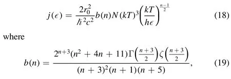
where ζ(x)is the Riemann ζ function and Γ(x)is the γ function.We find the index of the Compton spectrum is (n-1)/2 obtained by Equation(18)Thus,the hardest spectrum could be obtained Γ～0 when n →1,which corresponds the compression,C,to be a very large value based on Equation(11).This is impossible,but it give a mechanism to obtain a harder spectrum in the hot corona.The photon index of Γ=1.65 obtained by using the double warm model implies the compression equal to be about 2,which means the downstream density of shock is two times larger than the upstream density in the magnetic reconnection.It is noted that the hot corona is considered to be made of thermal electrons generally,but we replace the thermal model,nthcomp,with a simple power-law model,to obtain a similar photon index,which means that the hot corona radiation could be generated by a non-thermal process.

5.3.The Broad Fe Kα Line

If the double warm corona is true,the broad Fe Kα line should not be exist because the relativistic reflection component is excluded through the spectral analysis.However,both AG14 and Xu21 reported showing the broad Fe Kα line.We also test the Chi-square values of 4–10 keV by using the warm corona and reflection model,χ2=425 for warm corona model and χ2=414 for reflection model,which implies that the relativistic effect should be considered and the broad Fe Kα line should be exist.However,the X-ray spectrum of some AGNs with the reported broad Fe Kα line had been modeled successfully with narrow lines,and the complexity of reflection continuum could lead to a broad-line interpretation (e.g.,Murphy &Nowak 2014;Yaqoob et al.2016 and the recent work,Tzanavaris et al.2021),which means that the narrow emission is sufficient to model the broad Fe Kα line.The origin of the broad Fe Kα line is beyond the scope of this paper,so the broad Fe Kα line origin of ESO 362-G18 needs to be studied deeply in the future work.

5.4.The X-Ray Emitting Region

AG14 proposed that the X-ray radiation region is located within 50 rgby analyzing the absorption variability with 2005–2010 multi-epoch X-ray observations.The scale of 50 rgcorresponds to 104lt-s and the corresponding frequency is 10-4Hz which is simply within the middle frequency mentioned in Section.3.From the middle panel of Figure 6,there are no clear lags below 3 keV of the middle frequency,but it has some leading at 3–5 keV with about 2 ks and then has some lag at a high energy,about 8–10 keV with about 2 ks,which is the reverberation characteristics because 3–5 keV energy band represent the X-ray continuum radiated from hot corona to illuminate the disk and the lag at 8–10 keV could be a tail of“Compton hump.”The scale corresponding 2 ks is about9 rgwhich is less than the X-ray radiation region of 50 rg.The clear hard-lags shown at the low frequency appear to be～10 ks which corresponds 45 rgconsistent with the radiation region predicted by AG14.In Section 4,we find the double warm model could interpret the variability spectrum well.The second warm corona component is the main generation mechanism,and the hot corona and distant reflection dominate the radiation gradually at the high frequency,which means the warm corona component dominates the larger scale of the X-ray emitting region and the hot corona is mainly concentrated in the inner compact region which is consistent with the hypothesis that the hot corona is a compact source.The contribution of distant reflection at the high frequency could be considered as that the clouds in the distant reflection region have a small scale which corresponds the high frequency.

5.5.Exploring the Covariance Spectrum Property by Comparing with Time-average Spectra

The spectrometer of observation device is expected to try to find out the spectrum of a source.However,the spectrometer obtains is not the actual spectrum,but rather photon counts within specific instrument channels.This observed spectrum is related to the actual spectrum of the source as follows:

where C(I) is the photon counts within specific instrument channels,I;f(E) is the actual spectrum of the source;and R(I,E) is the instrumental response with units of cm2.However,f(E) cannot be determined by inverting Equation (20) due to the unstableness of C(I)(Arnaud 1996).The usual alternative is to try to choose a model spectrum,fb(E),that can be described in terms of a few parameters,and match,or fit it to the data obtained by the spectrometer.Therefore,the actual spectrum of the source depends on the choice of model.Then,we explore the covariance spectrum property by compared with the actual time-average spectra obtained by the Double Warm Corona model shown in Figure 23.The covariance data adopted are the same as Figure 9,but are divided by the scale of energy bin,which differs by one normalized factor from time-average spectrum because the response could be assumed a unit diagonal matrix for the covariance spectrum.Therefore,we adjust the normalized factor of covariance spectrum artificially to display the difference from the time-average spectra clearly in Figure 23.The blue solid line represents the continuum radiation of hot corona and the soft X-ray excess is apparent below 2 keV in the time-average spectra.Significantly,the soft X-ray excess of covariance spectrum is more prominent than that of time-average spectra in 0.5–2 keV,in which the second warm corona component is prominent.Below 0.5 keV,the soft X-ray excess of time-average spectra is stronger than that of covariance spectrum,in which the first warm corona component is prominent.So,the soft X-ray excess consists of the two warm corona components,but the variable degree of the first warm corona component is far less than the second.From Figure 23,we can see that the soft X-ray excess of covariance spectrum decreases gradually with frequency until none of the soft X-ray excess is shown in the high-frequency in which the variability mainly came from the hot corona.

5.6.Conclusions

We attempt to distinct between the warm corona and relativistic reflection models for the soft X-ray excess in ESO 362-G18 by using the simultaneous X-ray observation data of NuSTAR and XMM-Newton on 2016 September 24.We adopt five models including the warm,optically thick corona and relativistically blurred high-density reflection models,or their combination.The conclusions of this paper are as follows:

1.We find that the Double Warm Corona model can interpret both of time-average spectrum and variability spectrum (rms and covariance spectrum) well,which include the low,middle and high temporal frequencies.

2.The warm corona component is the main dominant mechanism in the low and middle temporal frequencies or a larger scale.The radiation of hot corona and distant reflection is dominant at high temporal frequency or a compacter scale.The distant reflection could be made of some moderate scale neutral clumps which corresponds the high temporal frequency.

3.The radiation mechanism of hot corona maybe comes from the non-thermal Comptonized process,such as the first order Fermi acceleration,to interpret the hard spectrum index obtained by the double warm model fitting.

4.If the double warm model is true,the broad Fe Kα line is absent because the relativistic reflection component is excluded through the spectral analysis.So the broad Fe Kα line origin of ESO 362-G18 needs to be studied deeply in the future work.

Acknowledgments

Thank the referee for their constructive comments.We acknowledge the financial supports from the National Natural Science Foundation of China (Grant Nos.11133006 and 11173054),the National Basic Research Program of China(973 Program 2009CB824800),and the Policy Research Program of Chinese Academy of Sciences (KJCX2-YW-T24).