Zhao Jianhua(赵建华),Wang Qiang,Wang Jin,Wang Ziqi,Zhang Bin,Chen Tao,Du Guojun,Gao Dianrong

(*Fluid Power Transmission and Control Laboratory,Yanshan University,Qinhuangdao 066004,P.R.China)

(**College of Civil Engineering and Mechanics,Yanshan University,Qinhuangdao 066004,P.R.China)

(***Jiangsu Provincial Key Laboratory of Advanced Manufacture and Process for Marine Mechanical Equipment,Zhenjiang 212003,P.R.China)

Abstract

Key words:magnetic-liquid double suspension bearing(MLDSB),nonlinear autonomous bearing system,equivalent nonlinear treatment,bearing performance indicator,parameter sensitivity,relative error

0 Introduction

Magnetic-liquid double suspension bearing(MLDSB)is mainly supported by electromagnetic suspension system and supplemented by hydrostatic bearing system,and then the phenomenons of poor load capacity,overload,seizing,bush-burning should be effectively avoided[1-5].

In recent years,many scholars have researched deeply on the nonlinear feature of hydrostatic bearing and electromagnetic suspension bearing, and have achieved fruitful research results.In Ref.[6],the nonlinear vibration of a single degree of freedom(DOF)rotor supported by active magnetic bearing(AMB)system was investigated.The typical nonlinear phenomena such as softening/hardening spring characteristic,jumps of the resonance curve can be observed and analyzed.In Ref.[7],the nonlinear dynamic behavior and stability of AMB-rotor system were studied by the Floquet theory.At the same time,the method consisting of a predictor-corrector mechanism and Netwon-Raphson method was presented to calculate critical speed corresponding to Hopf bifurcation point of the system.Ref.[8]showed that there were plenty of nonlinear phenomena such as periodic motion,almost periodic motion and chaotic motion in the process of system operation.Ref.[9]solved the nonlinear oil film force of the fixed-tilting tile sliding bearing by using the variational principle.And the influence of bearing fulcrum position and preload on the stability of the rotor was obtained by using point mapping and Runge-Kutta method analysis.Ref.[10]established the nonlinear axis of the trajectory mathematical model of four-oil cavity hydrostatic bearing.The influence of rotor speed,oil supply pressure and radius clearance of the bearing on the nonlinear axis locus is studied,and the change law of axis locus under dynamic load is calculated.

The electromagnetic suspension system and hydrostatic bearing system are inter-coupled,and the nonlinear degree of MLDSB is sharply increased.It is necessary to find a simple method which can be mastered by engineering designers and reflect the nonlinear features of MLDSB[11-12].

The equivalent linearization treatment is used to dispose single DOF bearing system of MLDSB.The mathematical expressions and sensitivity of parameters of equivalent stiffness/damping and the relative errors of stiffness/damping are obtained.Primary and secondary orders of bearing indicators of single DOF autonomous system are extracted,and the influencing rules of the major influence factors on the performance of MLDSB are revealed.Therefore,the research in the article can provide theoretical reference for the design and performance analysis of MLDSB.

1 Mathematical model

Eight magnetic poles are symmetrically distributed in the circumferential direction of MLDSB.And the adjacent opposite poles are a pair of magnetic poles.Initially,the electromagnetic force and hydrostatic force by each pair of magnetic poles are equal.A pair of magnetic poles are analyzed as a support unit.Single DOF bearing system in the vertical direction of MLDSB is taken as the research object.As shown in Fig.1,the bearing system is composed of rotor,upper and lower supporting units.

Fig.1 Force diagram of single DOF of MLDSB

In order to research the bearing performance of MLDSB,the assumptions are as follows[13-14].

(1)The flow state of the lubricant is laminar flow,and the liquid inertial force is ignored.

(2)The viscosity of the liquid is ignored.

(3)Leakage magnetic flux is ignored.

(4)The magnetic resistance in the core and rotor is ignored,and the magnetic potential is only applied to the air gap.

(5)The influences of hysteresis and eddy current of magnetic materials are ignored.

(6)Gravity of bearing and rotor are ignored.

The initial design parameters of MLDSB are shown in Table 1.

Table 1 Design parameters of MLDSB

1.1 Initial state of single DOF bearing system

In the initial state,the rotor is located in the rotation center of the bearing.And film thickness of upper and lower bearing cavities is equal.The bias voltage of proportional valve and the bias current of electromagnet are equal respectively.

Flow of proportional valve The initial bias voltage of the proportional valve is set tou0,and the output flow equation is as where,qf,0is output flow of proportional valve,L/min;k1is flow-voltage coefficient,L/min/V;u0is bias voltage of proportional valve,V.

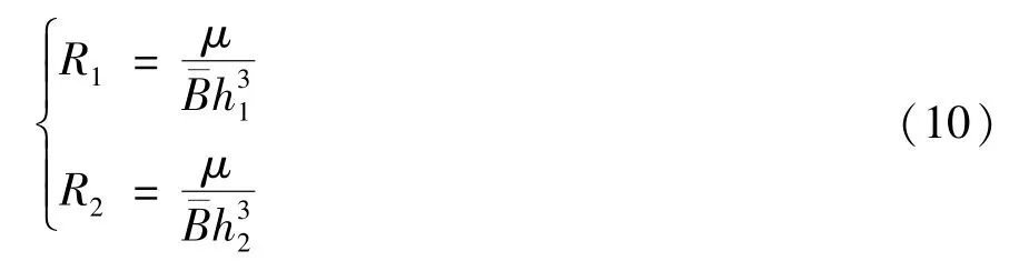
Liquid resistance of bearing cavity Upper and lower bearing cavities of MLDSB can be simplified as rectangular structures.The liquid resistance equations are obtained as

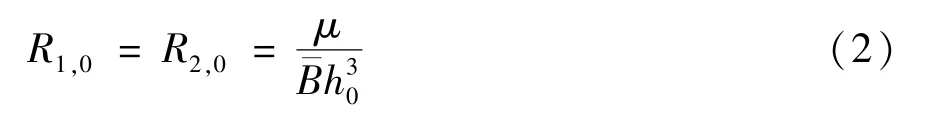
where,R0is liquid resistance of bearing cavity,Pa·s/m3;μis dynamic viscosity of lubricant,Pa·s;¯Bis bearing flow coefficient of bearing cavity,dimensionless;h0is film thickness of bearing cavity,m.

Hydrostatic bearing force According to Navier-Stokes equation[15],the hydrostatic bearing forces of upper and lower bearing cavities are obtained as

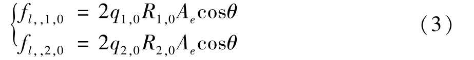
wherefl,0is hydrostatic bearing force of bearing cavity,N;q,0is input flow,L/min;Aeis effective bearing area,m2;θis angle between bearing cavity and center line of axis,°.

Electromagnetic bearing force According to Maxwell force equation[16],the electromagnetic suspension forces of upper and lower magnetic poles are obtained as

wherefe,0is electromagnetic suspension force of magnetic pole,N;kis electromagnetic constant,H·m,k=μ0N2A1/4;i0is bias current of solenoid,A;μ0is air permeability,H/m,μ0=4π×10-7;Nis coil turns,dimensionless;A1is iron core area,m2.

Flow balance equation Initially,the input flow of the bearing cavity is consistent with the output flow of the proportional valve.

whereq1,0is initial inflow of upper bearinng cavity,L/min;q2,0is initial inflow of underside bearing cavity,L/min.

Proportional equation of the suspension force

The proportional relationship between electromagnetic suspension force and hydrostatic bearing force is set to realize coupling support between two bearing systems.The proportional coefficient is assumed to beKas

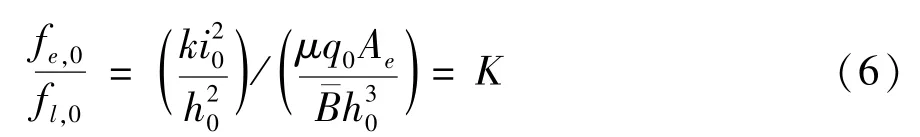
whereKis magnetic-liquid coefficient,dimensionless.

Mechanics balance equation According to Newton’s second law,and the mechanics balance equation of the rotor is obtained as

1.2 Working state of single DOF support system

Under the external load,displacement of rotor isx,and upper and lower film thickness areh1,h2respectively.

Flow of proportional valve The displacement of the rotor isx,and the direction is downward.The control voltage of coil of proportional valve isu.The flows of the valve are as

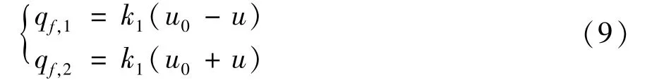
whereqfis output flow of proportional valve,L/min;uis control voltage,V.

Liquid resistance of bearing cavity When the film thicknesses of upper and lower bearing cavities areh1andh2,the liquid resistances of the bearing cavities are as

Hydrostatic bearing force According to Navier-Stokes equation,the hydrostatic bearing forces of upper and lower bearing cavities are obtained as

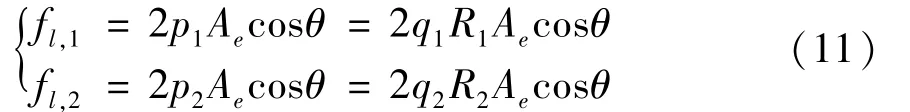
whereflis hydrostatic bearing force of bearing cavity,N;pis static pressure,Pa;qis input flow,L/min.

Electromagnetic suspension force According to Maxwell equation,the electromagnetic suspension forces of upper and lower magnetic poles are obtained as

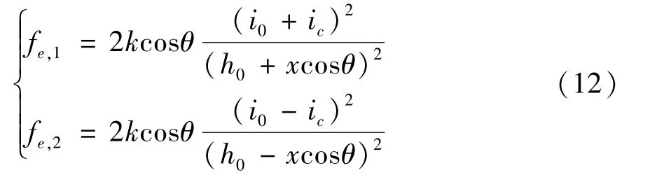
wherefeis electromagnetic suspension force,N;icis control current of solenoid,A.

Flow balance equation The influence of sensitive liquid path on bearing is ignored,and the flow balance equation between the bearing cavity and the proportional valve is obtained as

whereAbis the equivalent extrusion area of bearing cavity,m2.

Mechanics balance equation of rotor According to Newton’s second law,the mechanics banlance equation of the rotor is obtained as

wheremis rotor quality,kg.

1.3 Nonlinear autonomous equation of single DOF bearing system

Eq.(1)-Eq.(14)are comprehensively solved.Control voltageuof proportional valve and control current of solenoidicare assumed to be 0.The main parameters are shown in the Appendix 1.The dynamical equation of single DOF bearing system of MLDSB is obtained as

1.4 Linearization of dynamic equation

Taylor series expansion of the dynamic equation of single DOF bearing is carried out with the initial state as the reference.The dynamic equation of linearization is obtained as

2 Equivalent linearization and parametric sensitivity analysis

2.1 Equivalent linearization of dynamic equations

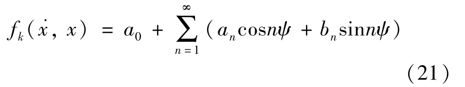
According to Eq.(15),damping force and elastic force of single DOF autonomous bearing system of MLDSB have strong nonlinear features.Firstly,an equivalent linearization dynamical equation corresponding to nonlinear autonomous equation of single DOF bearing system is established as

wheremeis equivalent quality,kg;ceis equivalent damping,N·s/m;keis equivalent stiffness,N/m.

Assume that the linear dynamical equation shown in Eq.(17)has stable periodic solution as follows.

whereatis equivalent amplitude,m;ωeis equivalent natural frequency, Hz;θ1is equivalent vibration phase,rad;ψis calculating parameter,dimensionless.

Eq.(18)is derived for timet,and the first and second derivatives are obtained as

Due to the low viscosity of seawater,the equivalent damping of single DOF autonomous bearing system of MLDSB is small.Therefore,amplitudeat,equivalent damping ratioδeand equivalent natural frequencyωein Eq.(18)and Eq.(19)can be expressed as

Substituting Eq.(22)into Eq.(17).

When the approximation of Eq.(18)and Eq.(19)is considered and constant forcea0is removed,Eq.(23)is expressed as

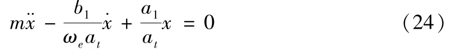
Equivalent massme,equivalent dampingceand equivalent stiffnesskeof single DOF autonomous bearing system are obtained by the equivalent linearization for Eq.(24).

Substituting Eq.(18),Eq.(19)and Eq.(26)into Eq.(25)as

Since there is an unknown quantityatin Eq.(27),equivalent dampingceand equivalent stiffnesskeare substituded into Eq.(20)as

Equivalent dampingcewill be replaced with linear dampingclas

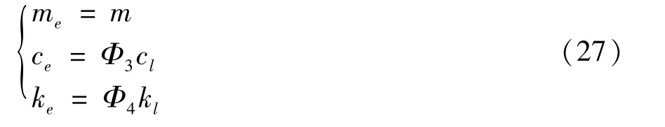
Substituting Eq.(29)into Eq.(27),and the expressions of equivalent massme,equivalent dampingce,and equivalent stiffnesskecan be obtained as

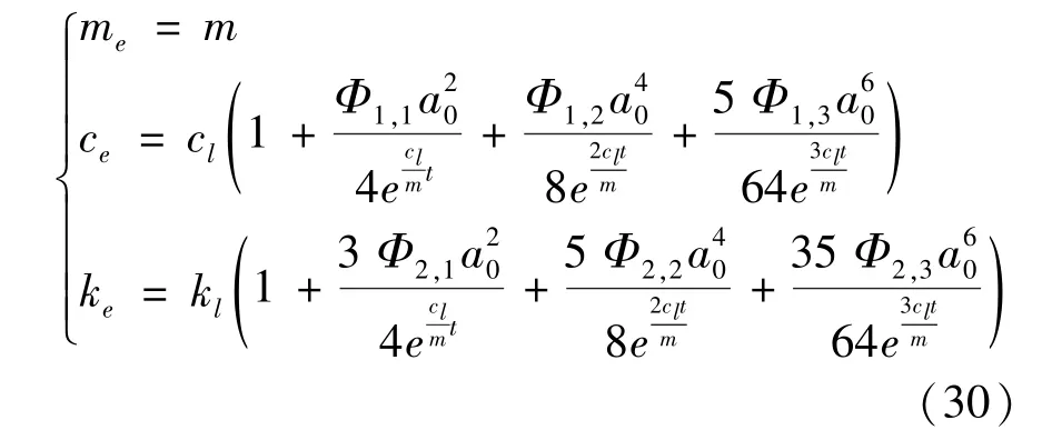
By comparing Eq.(16)with Eq.(30),equivalent massmeis rotor massm.And equivalent dampingce/equivalent stiffnesskeconsist of 4 parts respectively.First part is linear dampingcl/linear stiffnesskl,and the last three parts are high order minor terms which occurs during the process of Taylor series transform.

Substituting the parameters in Table 1 into Eq.(30),and the curves of linear damping,equivalent damping,linear stiffness and equivalent stiffness with timetare shown in Fig.2.

According to Fig.2,linear dampingcl/linear stiffnesskldoes not include timetand maintains constant.Equivalent dampingce/equivalent stiffnesskeof the first part is linear dampingcl/linear stiffnesskl.And the high order minor terms in the last three parts are positive eternally.

Fig.2 The curve of damping and stiffness with time

2.2 Sensitivity analysis of relative error of stiffness and damping

Definition of relative error According to Eq.(16)and Eq.(30),linear dampingcland linear stiffnessklare only related to the design parameters.Equivalent dampingceand equivalent stiffnesskeare not only influenced by design parameters,but also increases proportionally with timet.

Relative errorδkis defined to indicate the difference between equivalent damping/stiffness and linear damping/stiffness as follows.

Parameter sensitivity expression The relative error of stiffnessδkis expressed in the following form.

The expression of functiongin Eq.(32)is shown as

When the initial value of parameter vectorα0is constant,the initial value of state variableδk,0can be obtained as

In Eq.(34),the valueΔδkcan occur during the adjusting process of parameter vectorαas

Eq.(35)can be expanded by binary Talyor series expansion as

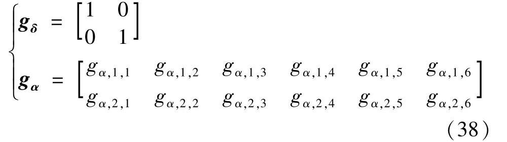
Substituting Eq.(32)-Eq.(35)into Eq.(36).

In Eq.(38),gδandgαrepresent second order Jacobian matrix(∂g/∂δ)and 2×6 order Jacobian matrix(∂g/∂α)respectively.

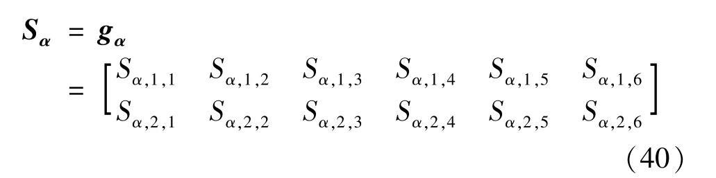
Eq.(37)can also be expressed in the following form.

Changing rule of relative error with time The relative errors of damping and stiffness are not only related to design parameters,but also demonstrate a trend of increasing first and decreasing with the time,as shown in Fig.3 and Fig.4.

Fig.3 Sensitivity of relative error of damping with time

Fig.4 Sensitivity of relative error of stiffness with time

3 Sensitivity analysis of bearing performances indicator

The influence of the relative error on the damping and stiffness of single DOF bearing system is mainly reflected in the change of the bearing performances of the autonomous bearing system of MLDSB.

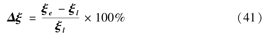
Sensitivity of relative error of bearing indicator The bearing indicators of linear and equivalent linearization are denoted by subscriptlande.And the relative errorΔξof two bearing indicators is obtained as

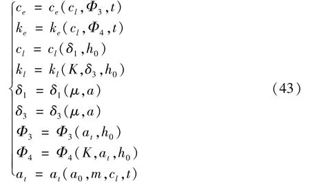
According to Eq.(39)-Eq.(43),the relative errorΔξof the bearing indicator is implicit function of the parametersm,kl,cl,ke,ce.

According to Eq.(16)and Eq.(31),ceandkeare implicit functions of parameterscl,klandФ10respectively.Andcl,kl,Ф10are implicit functions of parametersK,μ,a,a0,m,h0respectively.

According to Eq.(33)-Eq.(38),the sensitivity between the relative error of the bearing indicator and the design parameters is established as

whereχαis 5×6 order Jacobian matrix as

Influence of design parameters on relative errors Substituting the parameters in Table 1 into Eq.(45),the histogram of the relative error of bearing indicator with design parameter is obtained as shown in Fig.5.

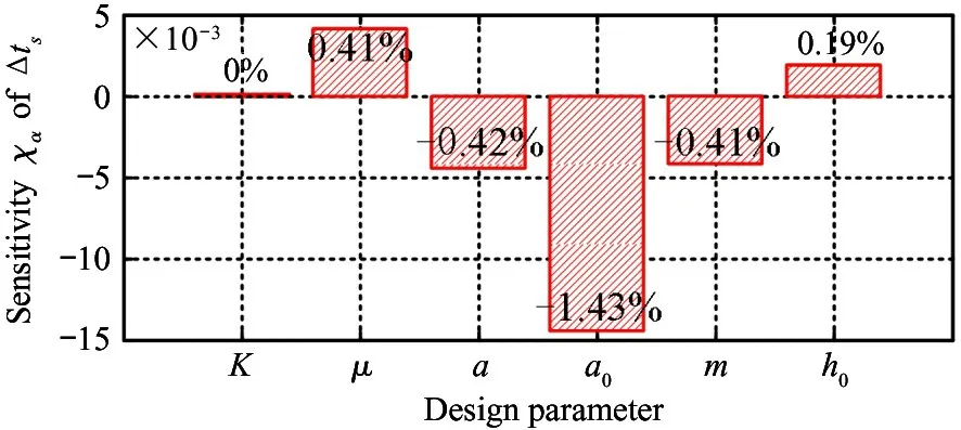
Fig.5 Sensitivity of relative error ofΔts(t=1 s)

According to Fig.5,the sensitivity of lubricant viscosityμand film thicknessh0to adjustment time is positive.It means that two parameters will lead to the increase of the adjustment time error.And the sensitivity of width of sealing sidea,rotor massm,and initial amplitudea0to adjustment time is negative.It means that 3 parameters will lead to the decrease of adjustment time error.The sensitivity of magnetic-liquid coefficientKto adjustment time is 0.It means that the error of adjustment time is not affected by the coefficientK.

According to Fig.6,the sensitivity of width of sealing sidea,initial amplitudea0and rotor massmto dynamic stiffness is positive.It means that the error of dynamic stiffness will increase with the parameters.The sensitivity of magnetic-liquid coefficientK,lubricant viscosityμand film thicknessh0to dynamic stiffness is negative.It means that the error of dynamic stiffness will decrease with the parameters.

Fig.6 Sensitivity of relative errorΔJ(t=1 s)

According to Fig.7,the sensitivity of magneticliquid proportionality coefficientK,lubricant viscosityμand width of sealing sideato phase margin is positive.It means that the parameters will lead to the increase of phase margin error.The sensitivity of initial amplitudea0,rotor massm,and film thicknessh0to phase margin is negative.It means that the parameters will lead to the decrease of phase margin error.

Fig.7 Sensitivity of relative errorΔγ(t=1 s)

4 Conclusions

(1)The sensitivity of relative error of damping and stiffness increases first and decreases with time,and the peak appears near 4 s.

(2)Initial amplitude is the major influence factor of natural frequency.Magnetic-liquid coefficient is the major influence factor of dynamic stiffness and phase margin.And film thickness is the major influence factor of amplitude coefficient.

(3)Film thickness and initial amplitude are the major influence factors of adjusting time,dynamic stiffness,phase margin,natural frequency and amplitude coefficient respectively.

(4)The sensitivity of relative error of adjustment time and natural frequency increases first and decreases with time,and then becomes stable.

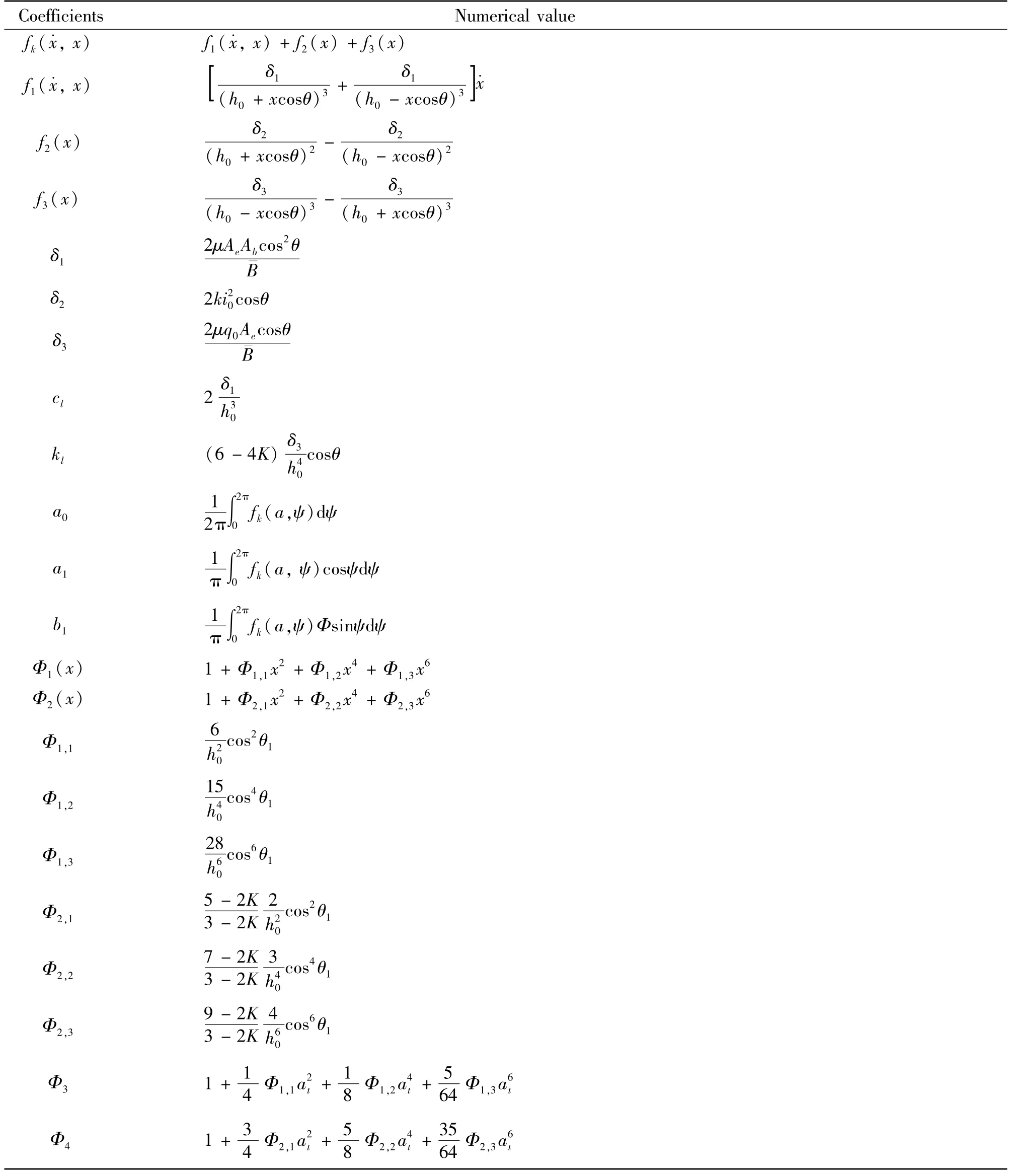
Appendix 1

Continued Appendix 1

Continued Appendix 1

Continued Appendix 1