Karthikeyan Rajagopal Anitha Karthikeyan and Balamurali Ramakrishnan

1Centre for Nonlinear Systems,Chennai Institute of Technology,Chennai,India

2Department of Electronics and Communication Engineering,Prathyusha Engineering College,Chennai,India

Keywords: discrete Josephson junction,fractional order,chaos,impulse control,chimera

1. Introduction

The invention of phase-locked loops (PLLs) in the early 20thcentury[1]has paved the way for their applications in various communication devices,and PLLs have attracted interest in recent years due to their rich nonlinear properties.[2,3]The simplest form of a continuous-time PLL consists of a voltagecontrolled oscillator and a phase detector in the feedback,and the PLL gets locked to the frequency when the phase error becomes constant.[4]A low-pass filter is usually used to remove high-frequency oscillations,[5,6]and the PLL with the filter is represented by a simple jerk system usually referred to as a third-order PLL model. Bifurcation and chaotic oscillations in these third-order PLLs are discussed where the route to crisis,periodicity,coexistence and their control are discussed.[7,8]

The analogue PLL has the drawback of DC drift and component precision problems, which limit their applications in sophisticated communication devices. Hence, discrete PLLs are preferred over analogue PLLs. In particular, the zero-crossing sampling discrete PLL (ZCSDPLL) is widely used. Nonlinear behavior of these ZCSDPLLs in their lower dimensions (first- and second-order) has been reported in Refs. [9,10] where the authors have also applied discrete PLLs for random number generation. Chaos and bifurcation phenomena in a third-order model of the ZCSDPLL was well reported in Ref.[11]where the authors have shown that ZCSDPLL exhibits periodic, quasi-periodic and chaotic oscillations for various parameter values. They have also shown that the ZCSDPLL a exhibits period-doubling route to chaos and disjoint chaotic attractors en route to chaos.

While the authors in Ref.[11]have discussed the chaotic behavior of the ZCSDPLL,they have done the analysis using a non-fractional difference equation. However,many earlier papers have shown that nonlinear systems that exhibit memory can be better analyzed using fractional calculus.[12–15]Nevertheless,all the fractional-order analyses of these memory systems use differential equations whose numerical solutions and solvers are well established. Since the ZCSDPLL is a discrete type,we use discrete fractional difference equations for analysis. There are not many references that discuss the control or network behavior of these ZCSDPLL systems.

In light of the above, we propose the fractional difference equation model of a ZCSDPLL.The bifurcation properties of the ZCSDPLL with respect to the fractional order and parameters are derived and presented to show the existence of periodic and chaotic regions. After proving the existence of chaos,we propose an impulse-based control algorithm and show efficient control regimes with respect to fractional order and impulse amplitude. To analyze the network behavior of the PLLs, we have construct a lattice network and study the synchronization of the PLLs in the network. Finally,we again use an impulse control method to suppress the chimera states and achieve complete synchronization of the nodes in the network.

2. Fractional-order discrete PLL

Since the invention of the phase-locked loop (PLL)in1932 by Bellescize,[1]PLL devices have found applications in many electronic and communication devices.[16]Even though the invention of PLL occurred as long ago as 1932, a mathematical model was only recently proposed.[17,18]Since then, there has been much interest in the investigation of the dynamics of PLLs. Many works have studied the nonlinear dynamics and existence of chaotic attractors in these PLLs.[19,20]However, most of these investigations have been on continuous-time PLLs, with far fewer on discrete-type PLLs, except for a few, as in Refs. [11,21]. The mathematical model of the discrete PLL (DPLL) proposed in Ref. [11]where the authors considered a zero-crossing digital phaselocked loop with a sampler,second-order loop digital filter and digitally controlled oscillator is given by

whereXdenotes the phase angle of the signal from the digitally controlled oscillator, anda,b,c,d,K, andrare the system parameters taken from Refs. [11,21]. The authors in Ref.[11]have discussed the chaotic behavior in the DPLL and have shown various bifurcations occurring in the DPLLs.

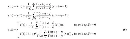
Much investigation has been dedicated to show that discrete fractional calculus is effective to analyze discrete nonlinear models,[22,23]and many methods have been proposed to solve the initial value problem of these discrete fractionalorder systems.[24]In this paper,we will derive the fractionalorder discrete PLL from Eq.(1)using the methods discussed in Ref.[25],whose general form may be expressed as

To numerically simulate Eq.(5),we use the discrete form(4)for each state variable and derive the dimensionless form for numerical analysis as

The 2D phase portraits of the FODPLL are shown in Fig.1 for initial conditions (x(0),y(0),z(0))=(0.1,0.1,0.1) and fractional orderq=0.01. The other parameters for the simulation area=3,b=−3,c=1,d=5.08,K=1, andr=2 and we use the definition in Eq. (5) to mathematically solve the FODPLL.

Remarks 1 To have a better range of simulations,we use the following relation in Ref.[25]:

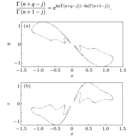
Fig. 1. Phase portraits of the FODPLL for q=0.01. Other simulation parameters are considered as a=3,b=−3,c=1,d=5.08,K=1,r=2.

3. Numerical analysis

The bifurcation analysis of a difference equation time discrete PLL was discussed in Ref. [8], where the authors have consideredKranddas the control parameters. When considering the FODPLL, we use fractional-orderqand parameterKas the control parameters and present the bifurcation diagrams. In Fig. 2, we show the bifurcation plot of the FODPLL with parameterKby keepingq= 0.05. ForK ≤1.523, the FODPLL exhibits a period-1 limit cycle oscillation and enters the first chaotic region for a small bandwidth of 1.523≤K ≤1.528. Then,the FODPLL enters three separate period-doubling routes and then the system enters a narrow period-1 oscillation region for 1.536≤K ≤1.54.When we compare this with Fig. 4 of Ref. [8], we see that the fractional-order discrete PLL exhibits a quasi-periodic region for 1.54≤K ≤1.545 and 1.55≤K ≤1.558. This quasiperiodic region was not seen in the original integer-order discrete PLL.[11]However,the quasi-periodic existence was well supported by Fig. 2 of Ref. [8], where the bifurcation of the discrete PLL withdexhibits regions of quasi-periodic oscillations. Hence, we confirm that fractional orders can enable us to investigate the unexplored behavior of complex systems. After the quasi-period region, the FODPLL goes into the second chaotic regime and exhibits chaotic oscillations tillK=1.62 and then goes unbounded.

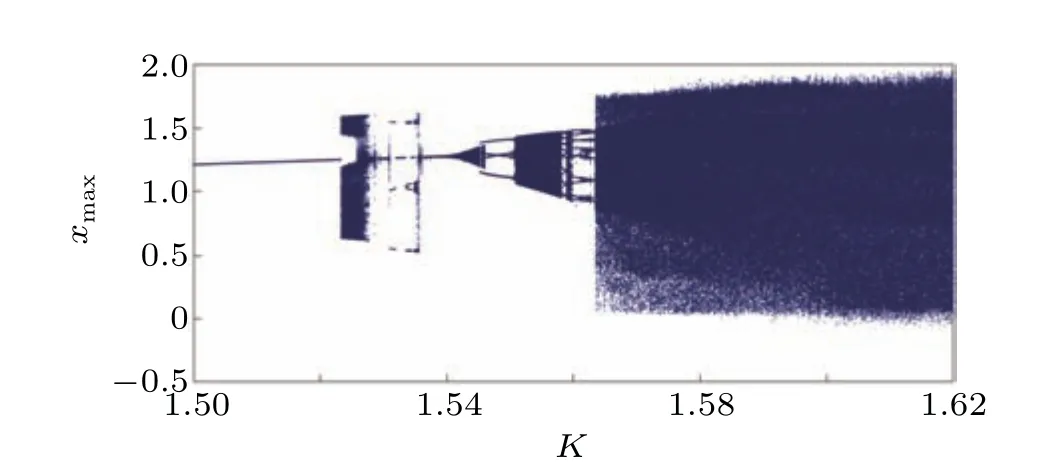
Fig. 2. Bifurcation of the FODPLL with K by fixing q=0.05. Other parameters are a=3, b=−3, c=1, d =5.08, r =2 and initial conditions[1,0,0].

In the second bifurcation discussion,we consider the fractional orderqas the control parameter and have fixedK=1.The value ofqis varied between[0.001,0.15].

To show the impact of the initial conditions,we have plotted the basins on thex–yplane where the red dots denote the chaotic regions and the white dots the periodic oscillations.For other values of initial conditions outside the regions covered by−0.5≤x(0)≤0.47 and−0.5≤y(0)≤0.5,the system goes unbounded.

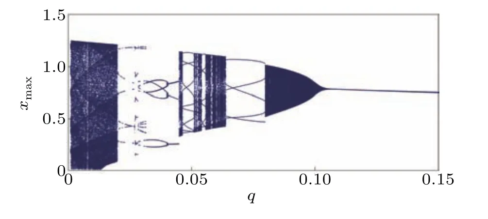
Fig.3. Bifurcation of the FODPLL with q by fixing K=1. Other parameters are a=3,b=−3,c=1,d=5.08,r=2 and initial conditions[1,0,0].

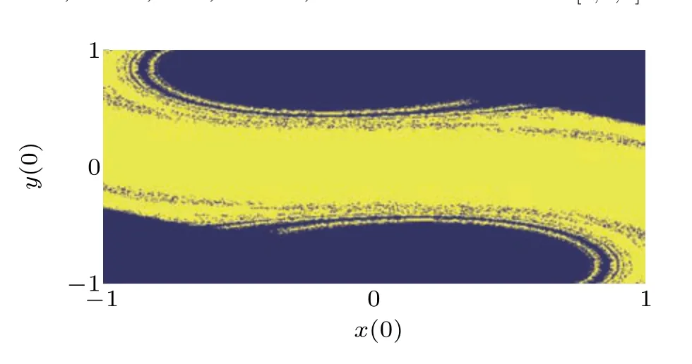
Fig.4. Basin of attraction of the FODPLL for q=0.01 and a=3,b=−3,c=1,d=5.08,r=2,K=1.

4. Chaos control of FODPLL

Having shown that the fractional-order discrete PLL has chaotic oscillations for selected values of fractional order and parameters, our goal is to introduce a method of chaos suppression using impulse control[25]as defined by

whereF(z)=az(k)+by(k)+cx(k)−dKsin(z(k))+K(1+r)sin(y(k))−Ksin(x(k)) fork=n+q −1. Parameterδis the step where we apply the impulse algorithm(6)andγis the impulse function. To understand the effect of the impulse control algorithm and to know the range ofγwhich can suppress the chaotic oscillations,we derive the bifurcation diagrams of the FODPLL with the control(6)against the various values ofγ. For this analysis, we choose various values ofδand plot the maximum value ofzas shown in Figs. 5–7. For all the bifurcation diagrams, we use forward continuation where we change the initial conditions to end values of state trajectories for every parameter setting.

In Fig.5,we consider that the control algorithm(6)is applied in every step andγis varied between [−0.2, 0.1]. We consider two fractional ordersq=0.01 shown in Fig.5(a)andq=0.05 shown in Fig.5(b). Forq=0.01,we can identify the effective control range ofγ ∈[−0.2,−0.12]shown in Fig.5(a)asγ1andγ2. Even though the control range can be considered for period-4 oscillation regions,we prefer period-1 oscillations as the other period oscillations have a smallerγrange and are also much closer to a quasi-periodic/chaotic region.Forq=0.05, the effective control range(period-1)of the algorithm shrinks toγ ∈[−0.2,−0.0713]and increasingqwill reduce the control range. We also note that there is no wider control window forγ>0 because when the impulse is applied to the present statez(n)the next state valuez(n+1)becomes(1+γ)z(n+1)thus making it higher than the actual value.[25]

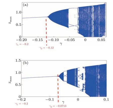
Fig.5.Bifurcation of the FODPLL against γ with the control applied in every step (δ =1) with (a) q=0.01 and (b) q=0.05 and a=3, b=−3, c=1,d=5.08,r=2,K=1.

Fig.6. Bifurcation of the FODPLL against γ with the control applied in every step (δ =2) with (a) q=0.01, (b) q=0.05 and a=3, b=−3, c=1,d=5.08,r=2,K=1.

Now,we consider that impulse control is applied at every two steps(δ=2),as shown in Figs.6(a)and 6(b)forq=0.01 andq=0.05 respectively. Forq=0.01, the control range isγ ∈[−0.2,−0.1387] and whenq=0.05, the control range isγ ∈[−0.4,−0.262]andγ ∈[−0.238,−0.226]. It is to be noted that forq=0.05,we can see two separate regions of period-1 oscillation one being wider and the second being a narrow one.

To further understand the impact of the step (δ) on the control ability, we have chosenδ=3,4,5 and plotted the bifurcation, as in Fig.7. In all the three cases, even though the system can be controlled to some periodic orbits, there is no period-1 limit cycle shown and hence, we can conclude that effective control can be achieved forδ=1,2.

Fig.7.Bifurcation of the FODPLL against γ with the control applied in every step,(a)δ =3,(b)δ =3,(c)δ =5 with q=0.01 and a=3,b=−3,c=1,d=5.08,r=2,K=1.

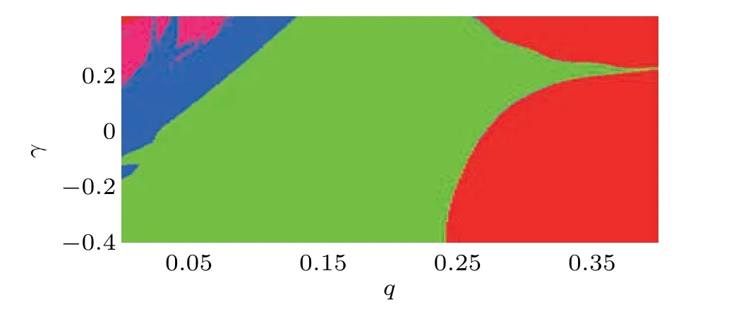
Fig.8. Various regions in a q–γ plane for q=0.01 and considering that the control is applied in every two steps(δ =2).

In Fig.8,we show the effective regions of control in aq–γplane consideringq=0.01 and the control applied in every two stepsδ=2. The green regions show the effective control area,the red region show the unbounded region,and the blue and the magenta shows different chaotic regions. It should be noted that the control region here refers to the numerically stable periodic oscillations.

Remark 1 In all the above discussion,we use the term periodic to mention the numerically stable periodic solutions.[25]As the fractional-order systems (continuous time) consider longer lengths of previous data (memory), there cannot be a constant periodic solution.[25,29]The same can be applied to fractional-order discrete systems too,and the periodic orbit referred to is a much closer trajectory to the periodic solution.

5. Spatiotemporal dynamics of FODPLL

Many kinds of electronic and communication equipment depend on discrete PLLs as they form their basic building blocks. Larger networks of FODPLLs are used in network applications, and the synchronization of the FODPLLs in these networks ensures efficient information processing.[26]The synchronization of these FODPLLs depends on the freerunning frequencies and each node phase detector gains.[27,28]Hence, our focus of interest is to study the behavior of the fractional-order discrete PLLs(FODPLL)in a non-locally lattice network,where we have assumed a ring connectivity with 2Pneighbours coupled as in

wherei=1 toNis the number of FODPLLs in the network,and in this simulation,we have takenN=200. For our analysis,we consider fractional orderqas the control parameter.We choose random initial conditions for the nodes in the network.

In our first discussion,we choose the fractional orders asq=0.01 and have captured snapshots of the network and final state of each node at the end of the simulation, as shown in Fig. 9. As can be seen from the figure, we can confirm that the nodes are in asynchronous states and do not show signs of synchrony. This is because the nodes are in chaotic states and since we use random initial conditions, the nodes never synchronize forq=0.01.

To confirm the asynchronous behavior of the system,we use the method described in Ref.[30],where the mean phase velocity is calculated by identifying the number of times(positive slope) the state variable crosses a constant. Using this method, we define the mean phase velocity of theN-th node asΩN=2πλ/T. Here,λdenotes the number of times the state variable crosses the constant with a positive slope andTdenotes the time interval.In Fig.10,we derive the mean phase velocity(MPV),and forq=0.01 shown in Fig.9 we confirm the asynchronous behavior in Fig.10 using the coherence circle plot and MPV plot. The number of coherent nodes(blue)is less than 0.5% of the total nodes, which confirms that the nodes are not synchronized.

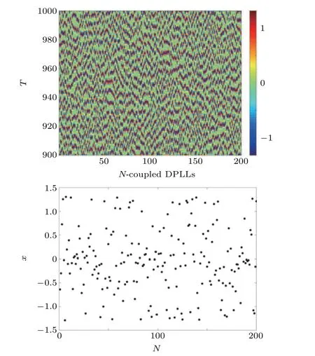
Fig. 9. Asynchronous behavior of the nodes in the network for q=0.01.State of each node at the end of the simulation is also shown.

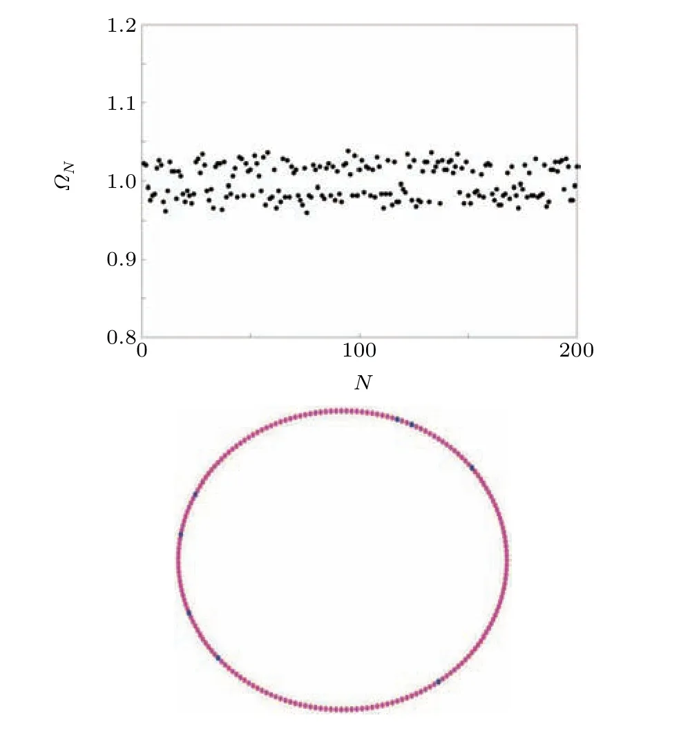
Fig.10. Mean phase velocity of the nodes for q=0.01;coherent circle plot where magenta denotes incoherent nodes,while blue denotes coherent nodes.

Fig.11. Chimera states of the nodes in the network for various values of fractional order. States of each node at the end of the simulation are also shown.

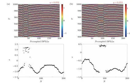
Fig.12. Chimera states of the nodes in the network for various values of fractional order. States of each node at the end of the simulation are also shown.

We now investigate the exact range of fractional orderq,responsible for chimera states and hence,we select a small range 0.05≤q ≤0.053 and capture spatiotemporal snapshots, as shown in Figs. 11 and 12. Since the coupling strength and other parameters are fixed so that the nodes are in a chaotic bursting state, we consider that the fractional order can initiate both coherent and incoherent nodes in the network. By fixingq=0.05,we note that most of the nodes are in the coherent state,while a few nodes are still in the asynchronous state. This is because of the multiple coexisting attractors, and since we have used random initial conditions, some nodes are driven to attractors that are located much farther away compared to the other nodes.To be exact, the nodes aroundi ∈[75.170] exhibit complete incoherency, while the other nodes are in the coherent state. By increasingqfurther to 0.051, the already synchronized nodes enter a much stronger coherent state and the number of coherent nodes increases.

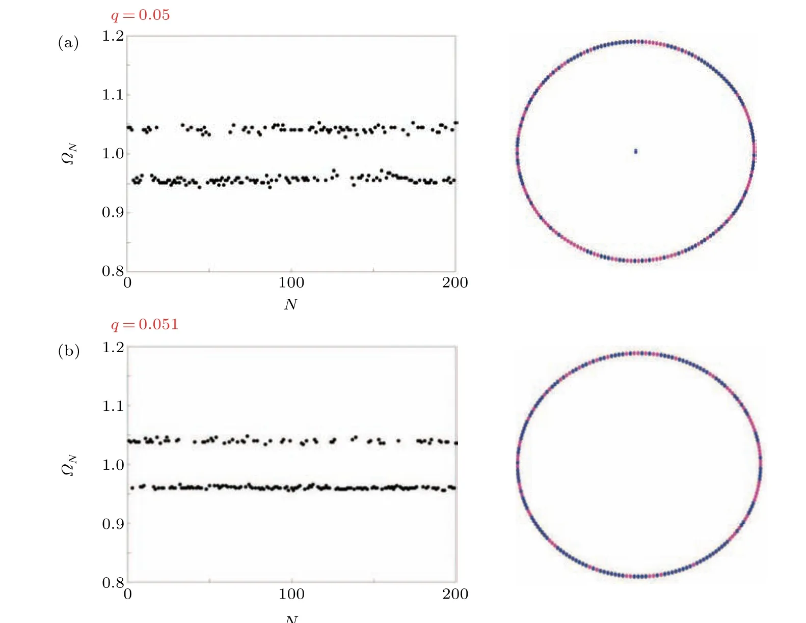
Fig.13. Mean phase velocity and circular coherency plots for different values of q.

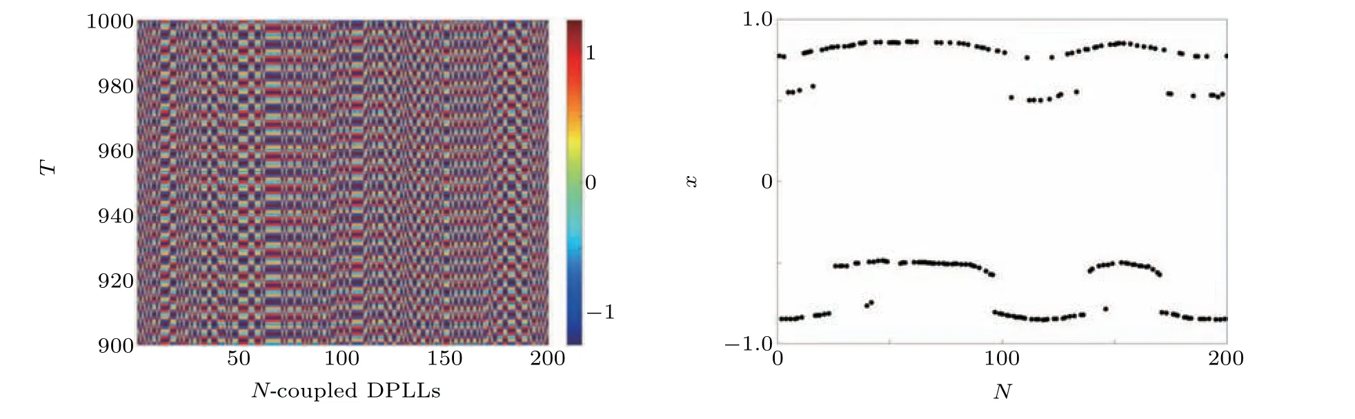
Fig.14. Cluster synchronization of the nodes in the network for q=0.07. State of each node at the end of the simulation is also shown.

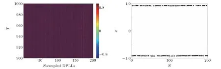
Fig.15. Synchronous behavior of the nodes in the network for q=0.15. State of each node at the end of the simulation is also shown.

By further increasing the fractional order toq=0.052,the coherent nodes increase in number compared to the incoherent nodes. Hence, the chimera states are preserved in the network. However, when the fractional order is kept atq=0.053,we can see that the number of incoherent nodes increases. This is because of the impact of fractional orderqfor which some nodes show coexisting behavior. These observations are clearly presented in Fig.12.

The MPV plots shown in Fig. 13 confirm the existence of chimeras in the network. Forq=0.051, the mean phase velocity of certain nodes is similar,which shows that they are in coherent states,while the incoherent nodes exhibit different MPVs. We use a circular coherence plot to show the coherent states(blue)and incoherent states(magenta). Around 70%of the nodes show coherent behavior,while 30%exhibit incoherency.Thus,we can confirm the existence of chimera states.

By further increasing the fractional order toq=0.07,the nodes start to synchronize and form local clusters with two on the positive amplitudes and two on the negative amplitudes,as in Fig. 14. This is because of the nodes entering a periodic region with period four limit cycles (refer Fig. 4) and hence,they cluster around four different amplitudes.

Complete synchronization of the nodes is achieved for fractional ordersq ≥0.1 as shown in Fig.15. The nodes synchronize to periodic positive and negative amplitudes depending on the initial conditions under which each node started. In this case, we consider random initial conditions ranging between[−0.1,0.1]so that we can have both positive and negative amplitude oscillations in the nodes.

6. Suppressing chimera using impulses

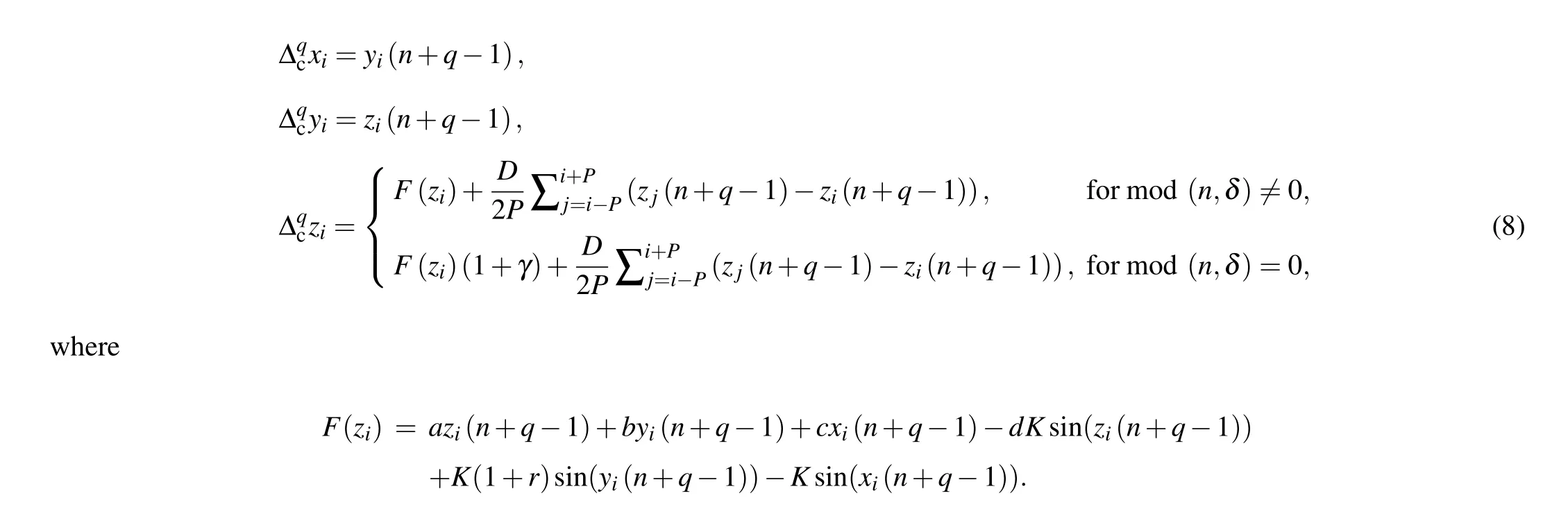
We show the existence of chimera states in the FODPLL network described by Eq.(7),and we now propose a technique to control the chimera states and achieve synchronization.The proposed control algorithm is like the one discussed in Eq.(8).The impulses of amplitudeγare applied to the nodes in the network whenn=δand the mathematical model used for the simulation is described as

We consider the same network setting as used in Section 5, and a fixed fractional order ofq=0.05 is considered for the entire analysis. In the first discussion, we consider a fixed control step (δ=2) and choose two values of the impulse function,as in Fig.16.

We start our investigation by selecting a positive value ofγclose toγ=0 and the nodes remain in asynchronous states,as can be seen in Fig. 16. We also showγ=0 to confirm that without control the network exhibits chimera states. We choose the negative values ofγsince its positive values cannot control the FODPLL(refer to Section 4). Forγ=−0.05,the nodes try to come towards synchronization(from complete asynchronous state refer Fig.9)and when we increase the impulse amplitude toγ=−0.1, the nodes are in an intermediate cluster synchronized form. Forγ=−0.2 a completely synchronized network exhibits that the proposed control algorithm is effective enough to bring to nodes from a complete asynchronous state to a complete synchronous state, as in Fig.17.

In the second discussion, we now fix the impulse amplitude toγ=−0.2 for which we have shown in Fig. 17 that complete synchronization is achieved and consider the control step as the parameter of discussion. For the values ofδ=1,2 the network remains in complete synchronized states, which corroborates our discussion in Section 4,as in Fig.18. When we consider higher steps,the nodes go into chaotic states and the network exhibits chimera-like behavior. Thus,we confirm that the control-step size plays a significant role in achieving local control and global synchronization.

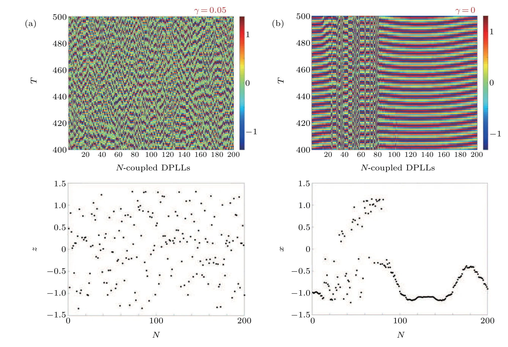
Fig. 16. Spatiotemporal behavior of the network (8) for various values of the impulse function γ. We consider that the impulse is applied every two steps. Value of the fractional order is considered as q=0.05.

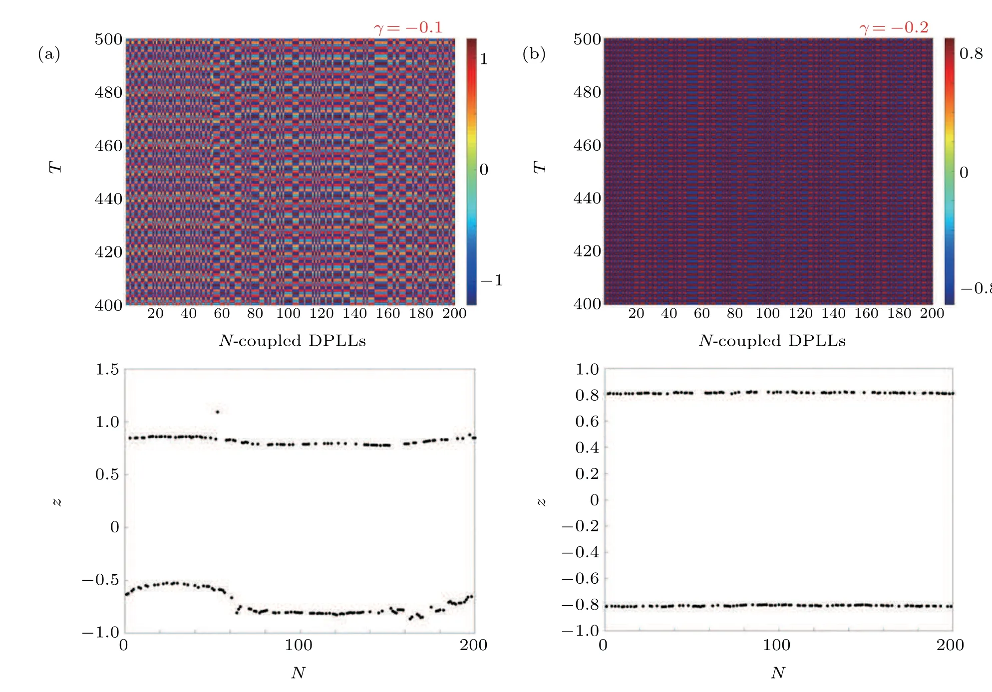
Fig.17. Spatiotemporal behavior of the network(8)for various values of the impulse function γ. We consider that the impulse is applied in every two steps. Value of the fractional order is considered as q=0.05.

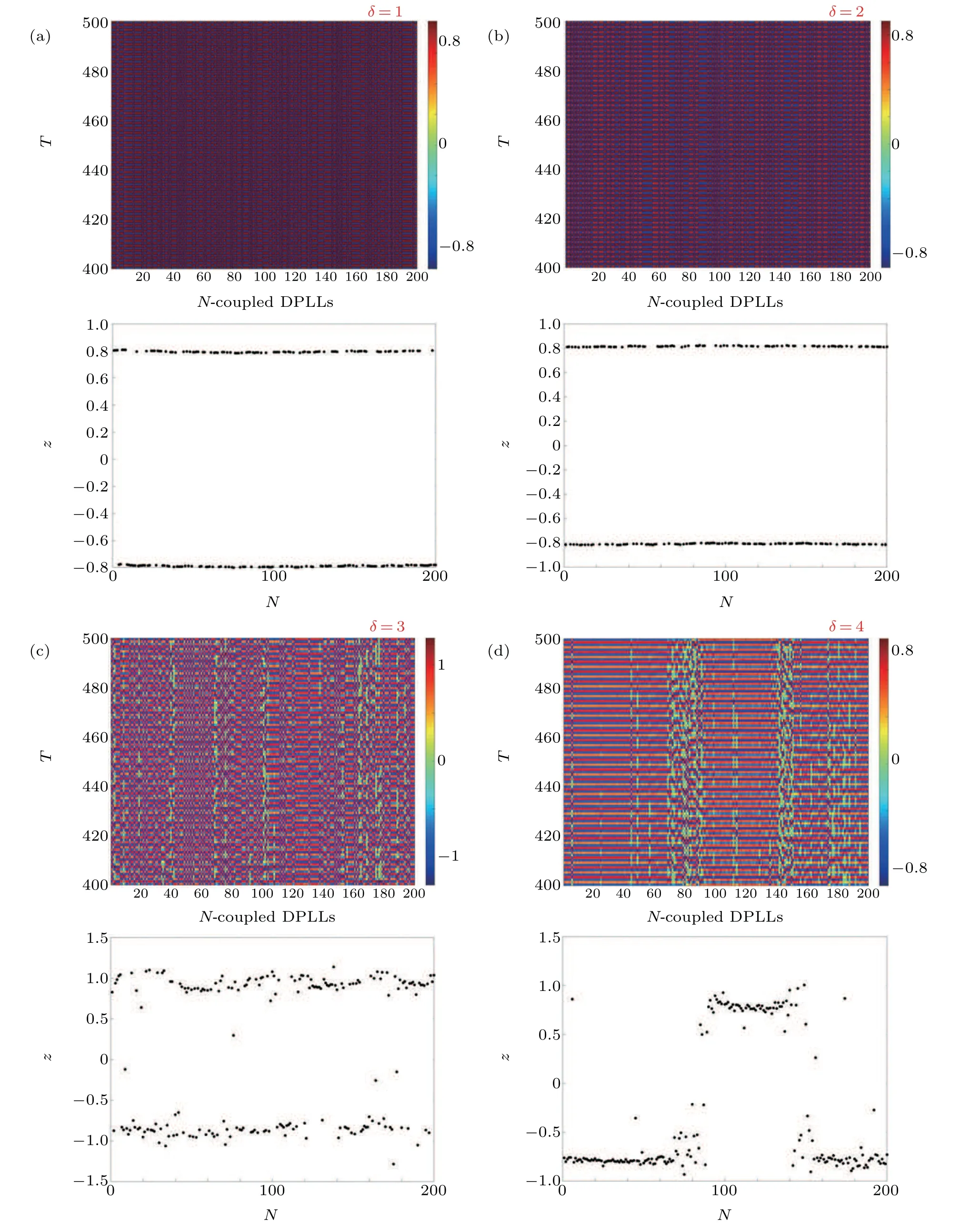
Fig.18. Spatiotemporal behavior of the network(8)for various values of the control step δ. We consider that the impulse amplitude is γ=−0.2. Values of the fractional order are considered as q=0.05.

7. Conclusion

In this paper,we model a fractional-order discrete phaselocked loop using a Caputo delta fractional operator, and we investigate the various dynamical properties of the FODPLL.Considering the loop gain (K) as the bifurcation parameter,we show the existence of a quasi-periodic region, which was not originally discussed in the integer-order ZCSDPLL model.Thus, by proving the existence of quasi-periodic and chaotic regions we now use the impulse control technique to suppress the chaotic oscillations. The lower control steps can suppress the chaotic oscillations better that the higher control steps. Furthermore, the positive impulse amplitudes cannot suppress the chaotic oscillations. The interdependence of the impulse amplitude (γ) and the fractional order (q) is investigated using a 2D plot on theγ–qplane. Investigating the network behavior of the FODPLL is of significance because of its applications in large-scale networks. For the analysis,we constructed a network of 200 FODPLLs and consider it as a ring network withPneighboring FODPLL. The network exhibits asynchronous behavior for lower fractional orders (q ≤0.03) and goes into complete synchronization forq ≥0.07. En route from asynchronous states to synchronous states, we see chimera-like behavior, especially in the range 0.049≤q ≤0.053. These chimera-like states are considered more hazardous in any physical circuits, and hence, we propose a simple control scheme to suppress these chimeras and achieve synchronization.An impulse function is applied to the individual nodes in the network everyδsteps,and forδ=1,2,we show effective suppression of chimera states. However,increasing the control steps further will strengthen the chimera states instead of controlling them. Hence,control steps play a vital role in achieving complete synchronization.