Quan Xu(徐权), Tong Liu(刘通), Cheng-Tao Feng(冯成涛), Han Bao(包涵),Hua-Gan Wu(武花干), and Bo-Cheng Bao(包伯成)

School of Microelectronics and Control Engineering,Changzhou University,Changzhou 213164,China

Keywords: extreme multistability,memristor,electromagnetic induction,Rulkov model

1. Introduction

The biological neurons play an essential role in electrical information dealing of nervous system.[1]Thus, it is important to disclose the dynamical prosperities of biological neurons in order to explore the mystery of nervous system. To date,diverse neuron models have been built to depict the main dynamical properties of neuron activities.[2]These neuron models can be mainly classified into two categories.One category is conductance-dependent neuron models, such as Hodgkin–Huxley model,[3]Morris–Lecar model,[4]Chay model,[5,6]and Wilson model,[7]which employs the electrophysiological characteristics of the cell membrane to reconstruct the ion channels to imitate the neuron activities.The other category is conductance-independent neuron models, i.e., Hindmarsh–Rose(HR)model,[8]FitzHugh–Nagumo model,[9]Izhikevich model,[10]and discrete Rulkov map,[11]which is constructed on dynamical assumptions to express the electrical activities of in-and out-signal without the consideration of neuron physiological structure. Most of these neuron models, no matter which categories they belong to, can generate rich electrical activities in response to externally applied stimulus,[12,13]electromagnetic induction,[14]and electromagnetic radiation.[15,16]That is to say, the neuron can realize its functions by feeling externally applied stimulus and conduction excitation of the change electrophysiology.[17,18]

To date, many explorations have revealed that externally applied stimulus and electromagnetic induction influence the dynamical properties of neuron electrical activities. By introducing an external applied current into HR model, various types of coexisting asymmetric bursters were disclosed.[12]And then,an external bipolar pulse current was imposed onto a two-dimensional(2D)HR model to imitate the periodic stimulus effect,from which the coexisting firing patterns have been explored.[13]Besides, the change of membrane potential during the exchange of intracellular ions and extracellular ions can lead to the variations of inner electrical field and induced current flow, and then a magnetic flow is induced.[19]Therefore,the effect of electromagnetic induction caused by the inner electrical field fluctuation should be considered in exploring the electrical activities of a neuron.[20]In other words,the electromagnetic induction participates and affects the electrical activity in a biological neuron. When modeling the neuron electrical activity with the consideration of electromagnetic induction effect, a flux-controlled memristor-enabled neuron model can be utilized for characterizing the electromagnetic induction effect.[21,22]The state equation of a flux-controlled memristor is restricted by the magnetic flux variation rate and applying voltage. Also,the memductance of a flux-controlled memristor is really dependent on its crossing flux.[23,24]These constraint relations of the flux-controlled memristor can effectively imitate the interaction between the electromagnetic induction effect and membrane potential of a biological neuron. Employing this scheme, many fascinating memristive neuron models have been raised and abundant electrical activities were numerically revealed.[25–28]

Inspired by the pioneer work, dynamical responses with different firing patterns and stochastic resonance were observed in the Hodgkin–Huxley neuron model by employing a flux-controlled memristor to emulate the electromagnetic induction flow.[29]The electromagnetic induction effects on the regulation of sleep wake cycle were further studied in a simple wake-sleep neural network coupled by glutamate synapse.It was found that the average firing frequency can be modified by the intensity of the electromagnetic induction.[30]And then, with comprehensive considerations of the electromagnetic induction and radiation, high and low frequency stimulus,and Gaussian white noise,mode transition of electrical activities and thought-provoking phenomena have been explored by bifurcation analysis.[31]To further reveal the effectiveness of electromagnetic treatment of mental diseases, the regulatory abilities of external electromagnetic stimulus on the dynamical properties of a small-world Newman–Watts network were explored.[32]Specially, the coexistence of spiking and bursting behaviors in a Leech neuron model was revealed and the synchronization of the two behaviors was investigated by coupling two identical Leech neurons.[33]After that,to mimic the threshold effect of electromagnetic induction, a threshold flux-controlled memristor-based HR neuron model was considered, from which the coexisting hidden bursting patterns were disclosed.[34]By building a locally memristive neuron model, the multistbility phenomenon was numerically simulated and experimentally captured.[35]The multistbility with multiple firing patterns was also disclosed in neural network coupled by memristive synapse, within which the memristor was utilized to express the electromagnetic induction induced by the difference of membrane potentials.[36–38]

The phenomenon of multistability has attractive great attention due to its potential use in the applications of image processing tasks.[33]Multistability involves various kinds of coexisting attractors for different initial conditions under fixed system parameters.[24,39]It is not easy to theoretically predict the multistability,but the initial condition offset-boosting and adoption of an ideal memristor are two empirical methods for acquiring multistability.[40,41]In general, multistability has been frequently found in autonomous systems,but has been rarely reported in non-autonomous one.[42]In this paper, by considering an externally injected alternating current and memristive electromagnetic induction effect,a continuous non-autonomous memristive Rulkov model is built. The phenomenon of extreme multistability is discovered in numerical and experimental surveys of the proposed model, which has not been reported in the state-of-the-art.

The two-dimensional (2D) discrete map-based Rulkov model was firstly established to imitate the dynamical properties of spiking and bursting firing patterns of a real biological neuron.[43]Then,numerous literatures have been published to numerically disclose the dynamical properties with different considerations.[44–47]The occurrence of multiple bifurcations was revealed in a non-chaotic Rulkov map with the consideration of delay.[44]Thereafter, coherence resonance and stochastic spiking-bursting excitability in the 2D Rulkov model with noise[45,46]and random force were numerically disclosed.[47]Beyond the work of single Rulkov neuron, Rulkov neuron-based networks with electrical and chemical synapse were built, from which the stability and chaos evolution,[48]synchronization of two identical and nonidentical Rulkov models,[49]and rich bursting patterns were numerically investigated.[50,51]All of these literatures were carried out in the numerical survey, but hardware implementation is more important for engineering application. Hardware implementation platforms can be divided into two categories, namely, analog hardware platform and digital hardware platform. Relatively speaking,analog hardware is one of the available way for the integrated circuit (IC) design,[52,53]which may promote a great convenience to engineering application of Rulkov model. Thus, a continuous Rulkov model is derived from the 2D map-based Rulkov model in this paper. Then, a continuous non-autonomous memristive Rulkov model is built by considering memristive electromagnetic induction and external stimulus. The electromagnetic induction flow is imitated by the generated current from a flux-controlled memristor and the external stimulus is injected using a sinusoidal current. The proposed Rulkov model can generate the novel phenomenon of extreme multistability with coexisting infinite firing patterns. The coexisting firing patterns in the proposed model can actually demonstrate multi-stable firing patterns emerging in biological neurons under the physical electrophysiological environment.

The remaining of this paper is arranged as follows. The continuous Rulkov model with the considerations of electromagnetic induction and external stimulus is built, and then the stability of the equilibrium point is numerically disclosed in Section 2. Parameter-associated dynamical behaviors are comprehensively explored in Section 3. Then, the extreme multistability depending on the initial conditions is further revealed in Section 4. Furthermore, the analog circuit-based hardware implementation and experimental measurement are executed in Section 5. Finally,the conclusion is drawn.

2. Model and equilibrium point stability

The 2D discrete map-based Rulkov model with a simple algebraic structure was firstly raised on dynamical assumptions of biological neurons.[43]It can reproduce periodic and chaotic spiking/bursting behaviors in biological neurons. Actually, a continuous nonlinear model is more efficient to reflect the dynamical property of a biological neuron due to its continuously dynamical evolution process. Thus, a continuous nonlinear model is derived by referring to the 2D discrete map-based Rulkov model. It can be mathematically written as

wherexrepresents the membrane potential andystands for the gating process.α,β,andσare three control parameters. Specially,σis employed to control the changing rate of the gating process andβis an externally applied influence.

Model(1)can only generate periodic behavior,because it is a 2D autonomous nonlinear model,i.e.,forα=11,σ=β=0.01, and initial conditions (x0,y0)=(0,0), model (1) generates a periodic spiking firing pattern. The phase trajectory and spiking firing pattern of the membrane potentialxare numerically simulated as shown in Fig.1. To exhibit its chaotic dynamics and to characterize the electrophysiology effects in the continuous Rulkov model, a continuous non-autonomous memristive Rulkov model is then built to address these issues.

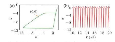
Fig. 1. (a) Phase trajectory and (b) spiking firing pattern of the membrane potential x for α = 11, σ = β = 0.01, and initial conditions(x0,y0)=(0,0).

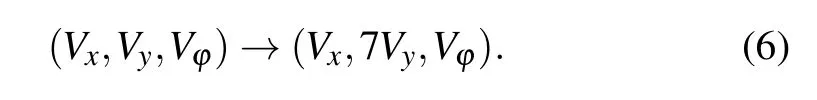
Herein,a flux-controlled memristor with quadratic memductanceW(ϕ) =a+bϕ2is employed to characterize the electromagnetic induction when neural activities are triggered.[34]Thus,with the simultaneous consideration of externally injected sinusoidal current and electromagnetic induction,a continuous non-autonomous memristive Rulkov model is built and written as

whereϕis the memristor inner state,k(a+bϕ2)xstands for the electromagnetic induction flow, andkindicates the coupling strength of the electromagnetic induction.Asin(2πFτ)is the externally injected sinusoidal current,in whichAandFare the amplitude and frequency, respectively. The effects of electromagnetic induction and external stimulus are simultaneously considered herein,which have been rarely involved in the literature.

Whenβ=0,model(2)possesses a line equilibrium set ofE=(¯x,¯y,¯ϕ)=(0,−α −Asin(2πFτ),c),within whichchas an arbitrary real value.Whereas,model(2)has no equilibrium point forβ/=0,which induces that model(2)generates hidden dynamics.[42]By numerous numerical simulations,it is found that model (2) generates transient periodic/chaotic behaviors but then tends to infinite in this case.[54]Thus,we mainly concern on the case ofβ=0 and select typical model parameters asα=11,σ=6,A=2,F=1,a=1,b=2,andk=0.1.

By linearizing model(2)around any equilibrium point ofE,the Jacobian matrix is obtained as

At the line equilibrium setE,the characteristic equation can be deduced as

Model (2) has a line equilibrium set evolving over the time. For the selected typical model parameters,the line equilibrium set is plotted in Fig. 2(a). Note that the value of ¯ϕfor the line equilibrium set is infinite and only illustrated in the region[−6,6]. Besides,the characteristic equation(4)has one zero eigenvalue and two nonzero eigenvalues. The stability of the line equilibrium set is really restricted by the model parametersa,b,σ,k, and the arbitrary real valuec. Whencis increased from−6 to 6 and parameterkis changed from 0 to 0.5 with other parameters fixed, the stability distribution of the line equilibrium set in thec–kplane is figured out in Fig. 2(b). The region I colored in blue has two positive real roots and the region II colored in yellow has a pair of complex conjugate roots with positive real parts. Different from these two regions, the region III colored in grey has a pair of complex conjugate roots with negative real parts. Summarily,I and II are two unstable regions,and III is stable region.Thus,model (2) can give birth to rich dynamics with the variations of parameterscandk.

Fig.2. Line equilibrium set and stability distributions for α =11,σ =6,A=2,F =1,a=1,b=2. (a)Line equilibrium set evolving over the time;(b)stability distributions restricted to the two nonzero eigenvalues in the c–k plane.

3. Parameter-associated dynamical behaviors

In this section, we select the model parametersk,α,A, andFas adjustable variables to explore the parameterassociated dynamical behaviors in model (2) numerically,

where MATLAB-based ODE23 algorithm with fixed time step 0.01 s and time interval[1.5 ks,2 ks]is used in plotting onedimensional (1D) and two-dimensional (2D) bifurcation diagrams. Besides, Wolf’s Jacobi method[55]with fixed time step 0.1 s and total time 10 ks is employed in depicting Lyapunov exponents and dynamical map. The initial conditions(x,y,ϕ)=(0,0,0)are assigned.

3.1. Parameters k and α related numerical plots

In this subsection, the dynamical behavior is fully disclosed by 2D bifurcation diagram depicted by checking the periodicities of the membrane potentialxand dynamical map described by the largest Lyapunov exponent in thek–αparameter plane as illustrated in Fig.3.

Fig.3. The 2D plots in k–α parameter plane with σ =6,A=2,F =1,a=1,b=2. (a)2D bifurcation diagram;(b)dynamical map.

In Fig. 3(a), the colormap is utilized to distinguish different dynamical behaviors,on which the red color labeled by CH denotes chaotic behaviors. The grey color labeled by UB denotes the unbounded behavior and the other colors labeled by P01–P08 represent the periodic behaviors with different periodicities of period-1 to period-8. Whereas in Fig. 3(b),the different colors on the colormap represent the values of the largest Lyapunov exponent, among which the deep red to white colors with the positive largest Lyapunov exponent denote chaotic behaviors, the black ones with the negative values present the periodic behaviors,and the grey color denotes the unbounded behavior. These numerical simulations explicitly disclose that the complex dynamics demonstrated by the 2D bifurcation diagram in Fig.3(a)well match those revealed by the dynamical map in Fig.3(b). These confirm the occurrence of complex dynamical behaviors in the continuous nonautonomous memristive Rulkov model(2)with the variations of the model parameterskandα. Note that model(2)goes to infinite with large model parameterαand strong electromagnetic induction of large coupling strength.

To more clearly reveal the dynamical evolution, the 1D bifurcation diagram and finite-time Lyapunov exponent are numerically simulated as shown in Fig. 4. Here, only the largest Lyapunov exponent is illustrated. Model (2) shows periodic and chaotic behaviors with the variations of parameterskandα, and these dynamical behaviors are confirmed by the corresponding finite-time Lyapunov exponents,respectively. Note that the finite-time Lyapunov exponents do not exist while model (2) running in unbounded behavior withk>0.3625 as shown in Fig. 4(b). The 1D bifurcation diagrams and finite-time Lyapunov exponent further confirm the complex dynamics in model(2).

Fig.4. The 1D bifurcation diagrams(up)and largest Lyapunov exponent(bottom)with the changes of(a)α and(b)k.

3.2. External stimulus related numerical plots

To disclose the dynamical behavior associated to the externally injected stimulus,we consider the stimulus related parametersAandFas two adjustable parameters while other parameters are taken as the typical ones. The 2D bifurcation diagram and dynamical map in theA–Fparameter plane are depicted in Fig.5. It is revealed that model(2)can generate rich dynamics with the changes of external stimulus related parameters. These reflect that the dynamical behaviors depend decisively on the externally injected stimulus.This can assistant us to understand the phenomenon of rapid mode transition under external stimulus in biological neuron. The dynamical behaviors revealed by 2D bifurcation diagram are basically coined with these disclosed by dynamical map. Note that model (2)tends to stable point attractor under small values ofAandFparameter region. The narrow parameter region locates at the left-down with white color in the 2D bifurcation diagram.

Fig.5. The 2D plots in A–F parameter plane with α =11,σ =6,k=0.2,a=1,b=2. (a)2D bifurcation diagram;(b)dynamical map.

Similarly,to more clearly reveal the dynamical evolution with respect to the external stimulus, the 1D bifurcation diagram and finite-time Lyapunov exponent are numerically simulated asAandFare changed respectively,as shown in Fig.6.Model(2)shows periodic and chaotic behaviors with the variations of parametersAandF,and these dynamical behaviors are confirmed by the finite-time Lyapunov exponents,respectively. The 1D bifurcation plots further reveal the stimulus related complex dynamical behaviors in model(2).

Fig.6. The 1D bifurcation diagrams(up)and largest Lyapunov exponent(bottom)with the variations of(a)A and(b)F.

4. Initial condition-associated extreme multistability

As a special kind of multistability, the phenomenon of extreme multistability happens with the number of coexisting attractors going to infinity. This special phenomenon has been first found in a memristive Chua’s circuit.[56]Then,initial-boosted extreme multistability in a two-memristorbased system[57]and hidden extreme multistability in a 5D system[58]have been revealed.In general,extreme multistability emerges in a system having an initial condition-associated perfect period-doubling bifurcation behavior. In this section,we mainly concern the initial condition-associated extreme multistability in model (2). The numerical simulations and colormap settings are identical with those utilized in Section 3.

4.1. Local attraction basin and dynamical map

The local attraction basins and dynamical maps inϕ0–y0andϕ0–x0initial condition planes are depicted in Figs. 7 and 8, respectively, which reveal that model (2) can generate rich initial condition-associated dynamical behaviors. The dynamical behaviors revealed by local attraction basin well coincide with these disclosed by dynamical maps. It is noted that the local attraction basin has the feature of inerratic strip structures.[59]This prominent feature implies that model (2)can easily generate a period-doubling bifurcation route by setting appropriate model parameters and initial conditions. The initial condition-associated period-doubling bifurcation route means the existence of extreme multistability,which indicates that model (2) can generate coexisting infinite firing patterns under the set of fixed model parameters. But the dynamical behavior does not alter with the initial conditionx0along with the initial conditionϕ0unchanging,as shown in Fig.8.

Fig.7. The 2D plots in ϕ0–y0 initial condition plane under the typical model parameters. (a)Local attraction basin;(b)dynamical map.

4.2. The 1D bifurcation plots

As predicted in Figs.7 and 8,extreme multistability and coexisting infinite firing patterns can be induced by taming the initial conditionsy0andϕ0. For better understanding,the 1D bifurcation plots are depicted in Fig.9. The initial conditions(0,y0,0)and(0,0,ϕ0)are employed in checking the extreme multistability with respect toy0andϕ0,respectively. In Fig.9(a),when the initial conditiony0increases from−2,the trajectory of model(2)begins with chaotic behavior.Then tangent bifurcation happens aty0=0.158,the trajectory runs into periodic behavior with period-5. Afterward, period-doubling bifurcation scenarios occur,the trajectory runs into chaotic behavior. The chaotic behavior extends toy0=1.484 and then tangent bifurcation happens again,the trajectory falls into periodic behavior. Thereafter, the period-doubling bifurcation scenarios occur again,leading model(2)to run in chaotic behavior.

Fig.8. The 2D plots in ϕ0–x0 initial condition plane under the typical model parameters. (a)Local attraction basin;(b)dynamical map.

Fig.9. The 1D bifurcation diagrams(up)and finite-time Lyapunov exponent(bottom)with the variations of(a)y0 and(b)ϕ0.

Fig.10. Phase trajectories(left)and time-domain waveforms(right)for different initial condition ϕ0. (a)Coexisting period-2 firing patterns for −2.2 and 1; (b)coexisting period-3 firing patterns for −1.5 and 1.45; (c)coexisting period-4 firing patterns for −0.5 and 1.36; (d)coexisting chaotic firing patterns for −2 and 0.5.

In Fig. 9(b), as the initial conditionϕ0increases from−3, the trajectory tends to infinite of unbounded behavior,then runs in chaotic behavior atϕ0=−2.295. Afterwards,the trajectory declines into periodic behaviors via perioddoubling bifurcations. Thereafter, chaotic crisis happens atϕ0=−2.183, then the trajectory runs in chaotic behavior.The chaotic behavior extends toϕ0=−1.705 and then the reverse period-doubling bifurcation scenarios occur, leading the model (2) to run in periodic behavior with period-3. After that, period-doubling bifurcation scenarios happen three times atϕ0=−0.618, 0.070, and 1.355, and tangent bifurcations happen two times atϕ0=0.028 and 0.675, leading to that model(2)runs into periodic behaviors and chaotic behaviors alternately. Lastly, the trajectory tends to infinite of unbounded behavior atϕ0=1.605. Clearly,extreme multistability and coexisting infinite firing patterns associated to the initial conditionsy0andϕ0are further confirmed by the 1D bifurcation diagrams and finite-time Lyapunov exponents as shown in Fig.9.

4.3. Phase trajectory and time-domain waveform

The phase trajectories and time-domain waveforms for some discrete values of initial conditionϕ0are plotted to further illustrate the extreme multistability with coexisting infinite firing patterns, as shown in Fig.10. Here, the fixed time step 0.01 s and time interval [1.9 ks, 2 ks] are employing in plotting the phase trajectory. The time interval [1.94 ks,2 ks]is employed in plotting time-domain waveform for more clearly visualization. The phase trajectories and time-domain waveforms for different initial conditionϕ0are illustrated in Figs.10(a)–10(d)respectively. It is revealed that the proposed model (2) can truly generate coexisting periodic and chaotic firing patterns. Actually, the firing patterns are non-standard spiking and bursting firing patterns. This reflect that the simultaneously considered electromagnetic induction and external stimulus can exert an influence on the dynamical properties of biological neurons.

5. Circuit implementation and experimental verification

The analog circuit implementation can involve the physical effects of parasitic circuit parameters for electronic neuron.Thus, the electronic neurons in analog form are significant to develop applications in artificial neural networks.[60]The model (2) can be equivalently realized by analog circuit.[1]The schematic of the equivalent circuit is given in Fig.11,the circuit equations for the three capacitor voltagesVx,Vy,andVϕare modeled as

whereVS=Vmsin(2π ft) is the input voltage to equivalently represent the externally injected current with the expression ofVS/R5,V1,V2are two direct voltages, andg1,g2,g3, andg4are the gains of the four multipliersM1,M2,M3, andM4, respectively.t=RCτis the physical time andRCis the integral time constant.

Since the dynamic range of the state variableVyexceeds the normal operation ranges of the active devices in Fig. 11,i.e.,operational amplifier AD711JN and multiplier AD633JN,a linear transformation should be made for decreasing the dynamic range ofVyin Eq.(5)as

Therefore, substituting Eq. (6) into Eq. (5) and comparing Eq. (5) with Eq. (2), as well as supposingV1=−1 V andV2=1 V,it yields

Suppose the integral time constantRC= 0.1 ms (i.e.,R=10 kΩ andC=10 nF) andg1=g2=g3=g4=1, the circuit parameters for the typical model parameters are calculated asR1=R5=R7=R8=R9=R10=R11=R12=R13=R14=R15=R17=R18=10 kΩ,R2=100 kΩ,R3=50 kΩ,R4=0.909 kΩ,R6=1.428 kΩ,R16=11.667 kΩ,Vm=2 V,andf=10 kHz.

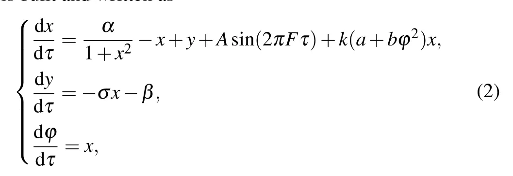
Refering to the circuit schematic in Fig. 11, an analog circuit is manually welded by commercially available discrete components on a printed circuit board. The monolithic capacitors and precise potentiometers,as well as the operational amplifiers AD711JN and multipliers AD633JN with±15 V voltage supplies are employed. The experimental results are captured by a Tektronix TDS 3054C digital oscilloscope in XY mode. To confirm the coexisting infinite firing patterns in the hardware experiment, the circuit parameters corresponding to the typical model parameters are employed. Only the resistanceR4in the analog circuit is adjusted to fine tune the hardware circuit. It is noted that the desired initial capacitor voltages are difficult to accurately acquire in the hardware circuit, which are randomly sensed through repeatedly turning on and off the hardware circuit power supplies.[24,36]The experimental resistanceR4= 0.752 kΩ, which is different from the theoritcal valueR4=0.909 kΩ. This deviation is caused by the model idealizations,parasitic parameters,measurement errors, and so on. Corresponding to the phase trajectories in Fig. 10, the coexisting infinite firing patterns are experimentally captured, as illustrated in Fig. 12. Besides,Fig.12 displays eight kinds of coexisting attractors for a fixed set of circuit parameters. For observability and to save space,these coexisting attractors are combined on the four figures by Photoshop processing.

Fig.11. Equivalent circuit implementations of the continuous non-autonomous memristive Rulkov model(bottom)and the memristor(up).

Fig. 12. Experimentally captured phase trajectories for random sensed initial conditions. (a) Coexisting period-2 firing patterns; (b) coexisting period-3 firing patterns;(c)coexisting period-4 firing patterns;(d)coexisting chaotic firing patterns.

6. Conclusions

In this paper, a continuous Rulkov model was firstly derived from the 2D discrete map-based Rulkov model, and then a continuous non-autonomous memristive Rulkov model was constructed by taking into account the memristive electromagnetic induction and externally injected sinusoidal current. Thus,the proposed model possesses a time-varying line equilibrium set. The time-varying line equilibrium set and their stability distributions were numerically simulated. It was specially revealed that the stability of the line equilibria set is not only dependent on the model parameters but also associated to the initial location of the memristor. These features can result in the generations of rich dynamical behaviors and extreme multistability. Multiple numerical methods were employed to disclose the dynamical behavior in the Rulkov model,which revealed the generation of chaotic behavior and periodic behavior with different periodicities, as well as rich mode transition behaviors. Besides,the extreme multistability with coexisting infinitely firing patterns was numerically explored. These numerical explorations reflect that the memristive electromagnetic induction and external stimulus can trigger rich neuron dynamics in biological neuron.Moreover,analog circuit-based hardware experiments were executed, from which the phase trajectories were captured to verify the numerical simulations. Particularly, the simultaneously considered electromagnetic induction and external stimulus can lead to the occurrence of non-standard spiking and bursting firing patterns, which can better mirror the electrophysiological activities of biological neurons in complex electrophysiological environment.