Hao Zhang(张浩) Yunjie Xia(夏云杰) and Deyang Duan(段德洋)

1School of Physics and Physical Engineering,Qufu Normal University,Qufu 273165,China

2Shandong Provincial Key Laboratory of Laser Polarization and Information Technology,Research Institute of Laser,Qufu Normal University,Qufu 273165,China

Keywords: computational ghost imaging, compressed sensing, deep convolution generative adversarial network

1. Introduction

Ghost imaging (GI) uses the spatial correlation of the light field to indirectly obtain the object’s information.[1–3]In the GI setup, the light source is divided into two spatially related light beams: the reference beam and the object beam. The reference beam, which never interacts with the object, is measured by a multipixel detector with a spatial resolution (e.g., a charge-coupled device), and the object beam after illuminating the object is collected by a bucket detector without spatial resolution. By correlating the photocurrents from the above two detectors, the image of the object can be retrieved. GI has attracted considerable attention from researchers because it has many peculiar features,such as turbulence-free,[4,5]medical imaging,[6–8]and night vision.[9,10]

However, the two optical paths of the conventional GI limit its application. In 2008,Shapiro creatively proposed the computational ghost imaging(CGI)that simplified the original light paths.[11]In the scheme of CGI,the spatial distribution of the light field is modulated by a spatial light modulator(SLM).The distribution of the light field in the object plane can be calculated according to the diffraction theory.Thus,the reference light path is omitted.Because of the simple light path and high quality,[12]CGI is the most potential imaging scheme for the applications of radar[13,14]and remote sensing.[15,16]

After more than ten years,the theory and experiments of CGI have become mature. However, a crucial disadvantage hinders the application of CGI, i.e., CGI needs to process a large quantity of data to obtain a high-quality reconstructed image. Compressed sensing (CS) provides an elegant framework to improve the performance of CGI, but its application has been restricted by the strong assumption of sparsity and costly reconstruction process.[17–20]Recently, deep learning(DL) has removed the constraint of sparsity, but reconstruction remains slow.[21–24]

In this article, we propose a novel CGI scheme with a deep compressed sensing (DCS) framework to improve the imaging quality. Compared with the conventional DL algorithm,neural networks in the DCS can be trained from scratch for both measuring and online reconstruction.[25]Here, we choose a CS based on a deep convolution generative adversarial network(DCGAN)to illustrate this method. Furthermore,we show a useful phenomenon in which background-noisefree images can be obtained by our method.

2. Theory

We depict the scheme of computational ghost imaging with deep compression sensing in Fig.1. In the setup,a quasimonochromatic laser is modulated by an SLM and then an objectT(ρ)is illuminated,and the reflected light carrying the object information is modulated by a spatial light modulator.A bucket detector collects the modulated lightEdi(ρ,t). Correspondingly,the calculated lightEci(ρ′,t)can be obtained by diffraction theory. By calculating the second-order correlation between the signal output by the bucket detector and the calculated signal, the object’s image can be reconstructed,[26,27]i.e.,

where〈·〉denotes an ensemble average. The subscripti=1,2,...,ndenotes theith measurement,andndenotes the total number of measurements. For simplicity, the object functionT(ρ)is contained inEdi(ρ,t).

Fig. 1. Setup of the computational ghost imaging system with a deep compressed sensing network.SLM:spatial light modulator,BD:bucket detector.

The flowchart of the DCS is shown in Fig.2. The model consists of four parts: (i) a CS program to compress the data collected by the CGI device,(ii)a conventional CGI algorithm,(iii)a generator G of DCGAN converts random data into sample images through continuous training;and(iv)a discriminator D of DCGAN distinguishes sample images from the real images.

Fig. 2. Network structure of the DCS. z represents random data; G(z)represents sample images; x represents real images, and the dotted arrows represent the iterative optimization process for the generator G and the discriminator D.

In the conventional CGI setup,a bucket detector collects a set of data(n). Correspondingly,the distribution of the idle light field in the object plane can be calculated according to the diffraction theory. Here, we can obtainn200×200 data points,and each data point can be divided into 20×20 blocks without overlapping. Under the CS theory,[17–19]the random Gaussian matrix is used to process the 20×20 data blocks,and a 400-dimensional column vector is obtained. In our scheme,the measurement rate is MR=0.25,so the size of the measurement matrix is 100×400. The process of CS can be expressed as

whereφ ∈RM×N(M ≪N) is the measurement basis matrix,x ∈RNrepresents the vectorized image block, andy ∈RMis the measurement vector.N/Mrepresents the measurement rate. Finally, we can obtain a 100-dimensional measurement vectorz.

By processing the above data with a conventional CGI algorithm,a new set of data(n)is obtained. Then,we train the data through a generator G of DCGAN. The network structure of generator G is shown in Fig. 3. The input is a 100-dimensional random vectorz. The first layer is the fully connected layer, and it turnszinto a 4×4×512-dimensional vector. The 2–5 layers are transposed convolution layers,and the number of channels is gradually reduced through the upsampling operation of transposed convolutions. In the second layer (a transposed convolution layer), 512×5×5 convolution kernels are used to generate 256×8×8 feature maps.The third network layer (a transposed convolution layer) is connected to the second layer, and 256×5×5 convolution kernels are used to generate128×16×16 characteristic graphs.The third layer of the network is connected to the fourth layer(a transposed convolution layer),and 128×5×5 convolution kernels are used to generate 64 32×32 feature maps.

Fig.3.Network structure of the generator G.FC:fully connected layer;TCONV:transposed convolution layer;512×5×5,represents the number and size of the convolution kernel; s represents stride(s); and pr represents pruning.

All the above processes are performed by batch normalization and the activation function is a ReLU(rectified linear unit) function. The fifth network layer (a transposed convolution layer) is connected to the fourth layer, and 64×5×5 convolution kernels are used to generate 3×64×64 feature maps. The activation function of the fifth layer is a tanh function. Finally,the sample images are output.

The sample images(3×64×64)obtained by the generator are used as input to the first layer. Then, the images go through a 50% dropout process to prevent overfitting so that the size of the image remains unchanged. The 3–7 layers are convolution layers. Figure 4 shows the discriminator network structure. In the third layer (a convolution layer), 3×5×5 convolution kernels are used to generate 64×32×32 feature maps. The third network layer is connected to the fourth layer(a convolution layer), and 64×5×5 convolution kernels are used to generate 128×16×16 feature maps.The fifth network layer(a convolution layer)is connected to the fourth layer,and 64×5×5 convolution kernels are used to generate 256×8×8 feature maps. The sixth network layer(a convolution layer)is connected to the fifth layer, and 256×5×5 convolution kernels are used to generate 512×4×4 feature maps. All the above processes are performed by batch normalization, and the activation function is a leaky ReLU function. The seventh network layer (a convolution layer) is connected to the sixth layer,and 512×5×5 convolution kernels are used to generate 1 scalar value.In this article, we choose TensorFlow as the learning framework and train the DCS model based on the TensorFlow learning framework. The learning rate is set to 0.0002,and the number of epochs is 500. The cyclic process can be described as follows: firstly, generatorGgenerates the sample images,then discriminatorDdiscriminates, and the loss is calculated by the output of generatorGand discriminatorD. Therefore,the loss function can be expressed as

Fig.4.Network structure of discriminator D.CONV:convolution layer;3×5×5 represent the number and size of the convolution kernel;s represents stride(s); pa represents padding.

whereDrepresents discriminatorD,Grepresents generatorG,xis the input to the model,G(x)represents the sample images andD(x) represents the probability thatxcomes from a real sample and does not come from a sample. Finally, the back-propagation algorithm is used to optimize the weight parameters, and then the next cycle is started. The test images are output every 25 epochs.

3. Results

The experimental setup is schematically shown in Fig.1.A standard monochromatic laser(30 mW,Changchun New Industries Optoelectronics Technology Co.,Ltd. MGL-III-532)with wavelengthλ= 532 nm illuminates a cube. A twodimensional amplitude-only ferroelectric liquid crystal spatial light modulator(Meadowlark Optics A512-450-850)with 512×512 addressable 15µm×15µm pixels through the lens collects the reflected light from the object. A bucket detector collects the modulated light. Correspondingly, the reference signal can be obtained through MATLAB software. The ghost image is reconstructed by the DCS. In this experiment, the sampling rate is MR=0.25 and the number of frames is 100.

Figure 5 shows a series of reconstructed images. Figure 5(a) is the object. Figures 5(b)–5(e) represent reconstructed ghost images with different numbers of frames. The experimental results obviously show that the reconstructed image quality is improved significantly with the increase in frames. The high-quality reconstructed ghost images are comparable to those of classical optical imaging with very little sample data.

Fig.5. The ghost image reconstructed by computational ghost imaging with compressed sensing based on a deep convolution generative adversarial network (DCS). (a) Real image. The numbers of frames in the reconstructed ghost images are(b)20,(c)40,(d)60,(e)80.

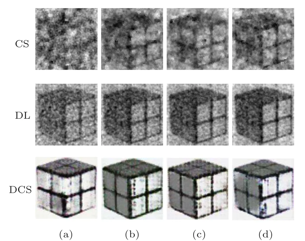
Fig. 6. Detailed comparison between reconstructed ghost images using the conventional compressed sensing (CS) algorithm, deep learning(DL)algorithm and deep compressed sensing algorithm(DCS).The numbers of frames in the reconstructed ghost images are(a)20,(b)40,(c)60,and(d)80.

We compare the conventional CS, DL, and DCS algorithms based on the same experimental data. The conventional CS algorithm and DCS algorithm have the same sampling rate,i.e.,MR=0.25. The DL algorithm and DCS algorithm set the same training times, i.e., 100 times. Figure 6 shows that the reconstructed images obtained by our scheme have the best quality under the same number of frames. Figure 6 clearly shows that the background noise can be eliminated by the DCS scheme, which is better than the CS and DL methods.In the generated network, the background noise is eliminated by full convolution. After each convolution, the noise information is reduced, and the details of the image will be lost accordingly. However, the transposed convolution layers in generatorGcompensate for the detailed information. Moreover, because of the existence of a discriminatorDthat can distinguish the “true” image, this causes the generatorGto constantly adjust the parameters to produce images with high reconstruction quality and low background noise.[28]

The peak signal-to-noise ratio(PSNR)and structural similarity index(SSIM)are used as evaluation indexes to quantitatively analyse the reconstructed image quality. The quantitative results(Fig.7)show that the PSNR of CGI with DCS is on average 57.69%higher than that of CGI with DL under the same reconstructed frame number, SSIM increased by 125%on average. More important, the image quality reconstructed by this method is much higher than that of the other two methods.

Fig.7. The(a)PSNR and(b)SSIM curves of reconstructed images of CS,DL and DCS with different numbers of frames,respectively.

4. Summary

Computational ghost imaging with deep compressed sensing is demonstrated in this article. We show that the imaging quality of CGI can be significantly improved by our approach. More important, this method can eliminate background noise very well,which is difficult for CS and conventional DL methods. The effect is more obvious, especially when the number of samples is small. Consequently, our scheme is more suitable for application in some special cases.For example, for fast-moving objects, we cannot collect a lot of data in a very short time.