Sixiao Kong(孔思晓) Chunbiao Li(李春彪) Shaobo He(贺少波)

Serdar C¸ic¸ek4, and Qiang Lai(赖强)5

1Jiangsu Collaborative Innovation Center of Atmospheric Environment and Equipment Technology(CICAEET),Nanjing University of Information Science&Technology,Nanjing 210044,China

2School of Artificial Intelligence,Nanjing University of Information Science&Technology,Nanjing 210044,China

3School of Physics and Electronics,Central South University,Changsha 410083,China

4Department of Electronic&Automation,Vocational School of Hacıbektas¸,Nevs¸ehir Hacı Bektas¸Veli University,Hacıbektas¸50800,Nevs¸ehir,Turkey

5School of Electrical and Automation Engineering,East China Jiaotong University,Nanchang 330013,China

Keywords: memristor,hyperchaos,coexisting attractors,amplitude control,neural network

1. Introduction

The memristor[1]as the fourth component is used to construct the connection between magnetic flux and electric charge in circuits. Because of this special nonlinear function, memristor has become a research hot spot in fields of chaotic oscillation and computing applications.[2-6]In a continuous nonlinear dynamic system,multistable attractors[7-14]can be extracted via flexible selection of the initial state,which brings great convenience to applications of chaotic engineering. Liet al.[15,16]introduced trigonometric functions for constructing self-reproducing chaotic systems. Based on the Sprott B system[17]or the four-dimensional autonomous system,[18]various types of coexisting attractors are studied.Multistability can be identified through offset-boosting,[19]since multiple coexisting attractors can be visited by changing the offset accordingly.[20,21]For those circuits and systems with memristors,[22-28]complex chaotic behavior with extreme multistability can also be found. Even in discrete systems, the memristor still gives its nonlinearity for producing chaos.[29]Inspired by the continuous memristor, and discrete memristor in the literature,[30-33]discrete memristor and trigonometric functions are introduced in a discrete map for more possible hidden features. As a result, in this work, it is found that the introduction of discrete memristor and trigonometric functions can give complex dynamics including multistability in a discrete map. More regimes of coexistence, especially coexisting chaotic and hyperchaotic attractors,under different Lyapunov exponents are expected by this exaggerated nonlinear introduction.

On the other hand, chaotic sequences also have great potential in radar and communication systems as continuous chaotic signals. For each application, the scale of a discrete sequence should meet the requirement of the integrated application system. Therefore, it is also important to control the discrete sequence accordingly. To the best of our knowledge,the amplitude control and offset-boosting of discrete mapping have not received enough attention even though they have been well studied in continuous systems. There is no related report on geometric control in discrete maps so far. For this reason,research of the control of amplitude and offset in chaotic maps is carried out.

Furthermore, in the rapidly developing field of artificial intelligence, the research in this field has been gradually extended to nonlinear science including prediction of the solution from continuous chaotic systems and discrete maps. For predicting chaotic signal, Alataset al.introduced chaotic particle swarm optimization algorithm[34]and whale optimization algorithm.[35]In addition, the genetic algorithm is also introduced in chaotic systems.[36]Artificial neural network,[37-39]multistep neural network,[40]deep neural network,[41]and complex neural network[42]methods are also used for prediction of complex structures of nonlinear systems. Cryptography[43]and random number generators[44]further reflect the application of artificial intelligence in chaotic system engineering. It is often necessary to extract or recover the chaotic signal or sequences in a chaos application. The traditional approach for signal reconstruction is based on chaos synchronization.[45-47]As a new alternative way, here the prediction of hyperchaotic and chaotic sequences based on external factor input autoregressive neural network algorithm is technically realized for chaotic sequence reconstruction.

Aim to reveal the coexistence of heterogeneous attractors related to periodic trigonometric functions,a memristive map with multistability is designed in this paper, where the initial state of the memristor cannot be ignored for picking out the present solution. In Section 2, the discrete memristor model and the constructed hyperchaotic map are given, and the stability of fixed points is also analyzed.In Section 3,the bifurcation property and typical phase trajectories are demonstrated.In Section 4, the multistability of the system is analyzed. In Section 5, the offset and amplitude control are discussed to further reveal the dynamic behavior of the system. In Section 6,the hyperchaos and other coexisting solutions are well predicted based on the NARX neural network(NARX:nonlinear auto-regressive model with exogenous inputs). Conclusions and discussions are given in the last section.

2. A 2-D memristive hyperchaotic map

2.1. A discrete memristor model

The preliminary idea of discretization of continuous memristors was proposed in Refs. [29,30]. According to the relationship of voltagev(t) and currenti(t), a magnetic fluxϕ(t)based on the forward Euler difference method,theni(t),ϕ(t) andv(t) are changed to beim,ϕm,vm, the memristor mathematical model is defined as follows:

whereϕm+1represents the(m+1)iteration of magnetic flux.For the following application, we leta= 1,b= 0.1 andk=0.4. In order to further prove the essential characteristics of the memristor,a discrete sinusoidal voltagevm=Asin(ωm)is selected as the terminal input. WhenA=0.1,ω=0.01,ϕ0=0 the hysteresis loop shows up, as shown in Fig. 1(a).The hysteresis loop changes like the issue in the continuous system when the amplitude or frequency of the input signal increases, as shown in Figs. 1(b) and 1(c). More strikingly,whenA=0.1,ω=0.01, andϕ0=−0.5,ϕ0=0,ϕ0=0.5,the hysteresis loops that depend on initial condition are shown in Fig. 1(d). The numerical simulation proves the essential characteristics of a memristor.[1]

Fig.1. The hysteresis loop of the discrete memristor(1)with sinusoidal input vm=Asin(ωm): (a)A=0.1,ω =0.01,ϕ0=0,(b)ω =0.01,ϕ0=0,(c)A=0.1,ϕ0=0,(d)A=0.1,ω =0.01.

2.2. A memristive hyperchaotic map

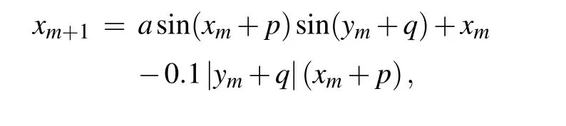
Introducing trigonometric functions into a nonlinear system can produce infinitely many coexisting attractors, while the memristor as a new nonlinear element can promote the complexity. Here, by introducing the discrete memristor and trigonometric function,and a new two-dimensional map is obtained as

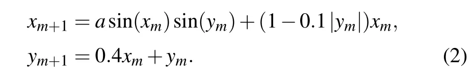
The memristorWis applied for restraining the internal variableyrather thanϕin Eq. (1), and now correspondingly the state variablexcan be regarded as the voltagev. Heremis a natural number(0,1,2,3...),xmandymrepresents them-th state value,ais a system parameter,anda=0.

2.3. Fixed point analysis

In the discrete map, the stability characteristics are usually characterized by fixed points. The fixed points (x∗,y∗)satisfy the equation

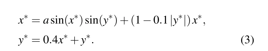
Therefore,

whereβis an arbitrary constant,and the Jacobian matrix corresponding to Eq.(4)is

Substituting Eq.(4)into Eq.(5),we have

The eigenvalueλ1= 1 always lies on the unit circle.Becausea= 0 andβis any nonzero real number,λ2< 1,which is always in the unit circle, implying that the fixed point is stable. For the casea=1, whenβis in the range of [−20,−5.619]∪[−3.441,0], the eigenvalueλ2≤1, the fixed point is within the unit circle; whenβis in the range of (−5.619,−3.441), the eigenvalueλ2>1, the fixed point is unstable. For the casea= 2, whenβis in the range of [−20,−17.69]∪[−16.65,−11.87]∪[−9.913,−5.926]∪[−3.253,0], the eigenvalueλ2≤1, the fixed point is in the unit circle; whenβis in the range of (−17.69,−16.65)∪(−11.87,−9.913)∪(−5.926,−3.253), the eigenvalueλ2>1, the fixed point is unstable. For the casea= 4,whenβis in the range of [−20,−18.3]∪[−16.04,−12.18]∪[−9.552,−6.088]∪[−3.189,0], the eigenvalueλ2< 1, and the fixed point is in the unit circle; whenβis in the range of(−18.3,−16.04)∪(−12.18,−9.552)∪(−6.088,−3.189),the eigenvalueλ2>1, the fixed point is unstable. In conclusion,the fixed points of the hyperchaotic map are critically stable or unstable, depending on the values ofaandβ, as shown in Fig.2.

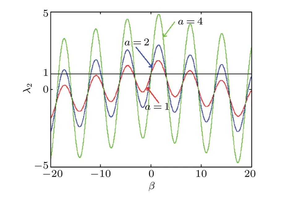
Fig.2. The second eigenvalue of the fixed point swings with the parameter a.

3. Bifurcation analysis

Let initial condition (x0,y0)=(1,−2), when the system parameterachanges in the range of[1,4.2],the bifurcation diagram and corresponding Lyapunov exponents are shown in Fig.3.

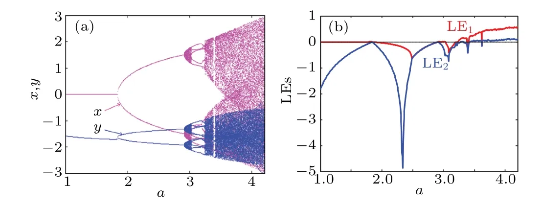
Fig. 3. Dynamical behavior of hyperchaotic map (2) under the initial condition (x0,y0)=(1,−2) when a varies in the range of [1,4.2]: (a)bifurcation diagram,(b)Lyapunov exponents.

When the parameteraincreases,a period-doubling bifurcation shows up. Chaos and hyperchaos become the dominant oscillation with occasionally periodic windows, some typical phase trajectories are shown in Fig. 4. Lyapunov exponents and Kaplan-Yorke dimension are calculated based on Wolf’s algorithm,as listed in Table 1. We can see that for the hyperchaotic attractors,all Lyapunov exponents are positive.

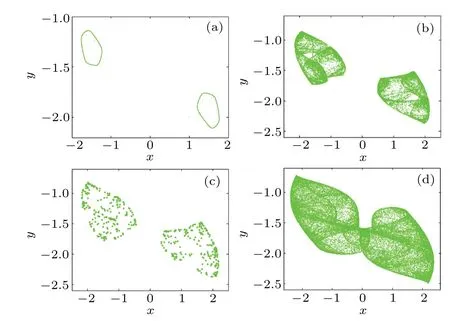
Fig.4. Typical phase trajectories of map(2)under the initial condition(x0,y0)=(1,−2): (a) a=3.00, closed quasi-periodic, (b) a=3.36,chaos,(c)a=3.40,discrete periodic points,(d)a=3.60,hyperchaos.

Table 1. Detailed analysis of typical phase trajectories of the map (2)under the initial condition(x0,y0)=(1,−2).

4. Coexisting chaos and hyperchaos

In the memristive map, there are many coexisting solutions for the existence of trigonometric function and memristor. To find those coexisting attractors, the bifurcation diagram depending on the variation of the initial state is explored.Meanwhile, the corresponding Lyapunov exponents are obtained. As shown in Fig. 5, when the initial state varies in a certain range,various coexisting solutions are observed. Besides coexisting chaos and hyperchaos, more strikingly, here in fact,various chaotic attractors and different hyperchaotic attractors coexist together,which has not been reported in other systems.

Typical phase portraits and the coexistence are displayed in Fig. 6 under the different parametersa. To get attractors more clearly, green, red, cyan and magenta, are selected to represent different phase trajectories. Four cases are considered in the following.

Case 1a=3.00. As shown in Fig. 6(a), there are four classes of attractors, which are hyperchaotic attractor, quasiperiodic curve, chaotic attractor, and discrete periodic points when the initial conditions are(1,−8),(1,−6),(1,0),(1,10).

Case 2a=3.36. As shown in Fig. 6(b), coexisting hyperchaotic attractors and chaotic attractors are seen when the initial conditions are(1,−18),(1,−12),(1,−5),(1,2).

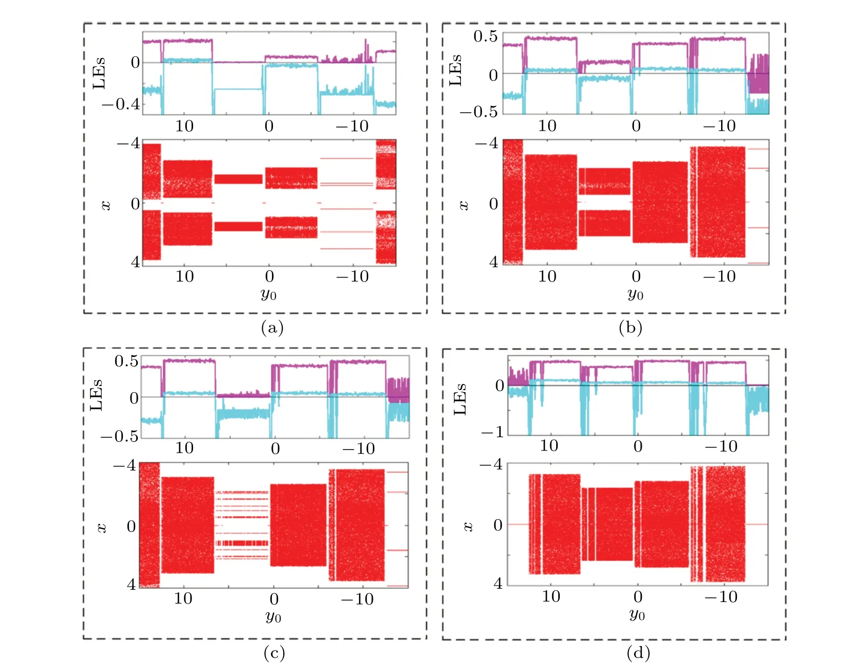
Fig.5. Dynamical behavior of map(2)under the initial condition(x0,y0)=(1,y0): (a)a=3.00,(b)a=3.36,(c)a=3.40,(d)a=3.60.

Case 3a=3.40. As shown in Fig.6(c),there are discrete periodic points,hyperchaotic attractors,and chaotic attractors when the initial conditions are(1,−4),(1,3),(1,10),(1,13).

Case 4a=3.60. As shown in Fig. 6(d), there are only coexisting chaotic attractors and hyperchaotic attractors when the initial conditions are(1,−10),(1,−6),(1,3),(1,9).

Fig.6. Various regimes of multistability in map(2): (a)a=3.00,(b)a=3.36,(c)a=3.40,(d)a=3.60.

All the above regimes of multistability can be indicated by the offset boosting under a fixed initial condition.[48]Suppose that the offset boosting is applied to the dimension ofy,

In this case, the fixed initial point will pass by the moving basins of attraction induced by the offset boosting, consequently,various coexisting attractors show up leading to a couple of jumps among different Lyapunov exponents, as shown in Fig.7. The frequently happened switches of Lyapunov exponents confirm the coexistence of multiple dynamics.

Fig.7. Multistability in map(9)detected by the offset boosting under the initial condition(x0,y0)=(1,−2), when q varies in[−10,10]: (a)a=3.00,(b)a=3.36,(c)a=3.40,(d)a=3.60.

5. Offset-boosting and amplitude control

The discrete map can be controlled in the offset and amplitude. Taking a substitution ofgx+p,hy+q(heregandhare for amplitude control,pandqare for offset boosting,g=0,h=0)in Eq.(2),

Unlike those continuous systems, to realize the offsetboosting in a discrete map it is necessary to introduce two offset boosters at both sides of the equation. In particular,when the amplitude control is realized in Eq.(10),the offset boosterspandqget coupled with the amplitude controller. As a special case, wheng=h=1, offset boosting can be realized via

As shown in Fig.8,whena=4.2 andp=q=0 are satisfied, the bipolar signal of the chaotic signalxandycan be obtained as shown in the green attractor. Due to the attracting domain of the system itself,adjusting the corresponding initial conditions (x0,y0) can help to get the offset of the attractor.Figure 8 gives the offset-boosting attractors in the dimension ofxandy. Corresponding waveforms are shown on the right,indicating that the offset can be switched flexibly from negative to positive. When the attractor is offset boosted,the corresponding basin of attraction shifts accordingly in phase space,as shown in Fig.9. Similarly,it can be seen from Fig.10 that the bifurcation diagram and Lyapunov exponents also illustrate the existence of offset-boosting.

Fig.8. The offset-boosted attractors in map(11)under the initial condition(x0,y0)=(1−p, −2−q):(a)x-dimension(cyan for p=8,q=0;green for p=0,q=0;magenta for p=−8,q=0),(b)y-dimension(red for p=0,q=4;green for p=0,q=0;blue for p=0,q=−4).

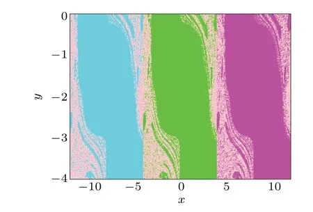
Fig.9.Shifted basin of attraction in hyperchaotic map(11)with a=4.2 in[−12, 12](cyan for p=8;green for p=0;magenta for p=−8).

Ignoring the offset constantsp,qand the amplitude controllerhin Eq.(10),a single amplitude control can be obtained in the dimension ofx,

As shown in Fig. 11, in thex-dimension, the constantgcontrols the amplitude of the hyperchaotic attractor. There is a certain relation between offset-boosting and amplitude control,which influences the depth in offset boosting.

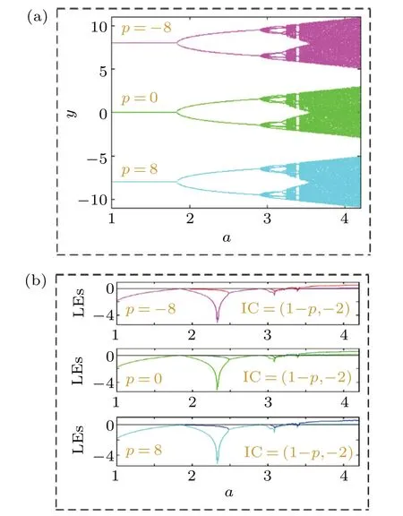
Fig. 10. Independent bifurcations in map (11) under different offset boosting when the initial condition (x0,y0) = (1 −p,−2) (cyan for p=8;green for p=0;magenta for p=−8): (a)bifurcation diagram,(b)Lyapunov exponents.

Fig.11. The hyperchaotic map(12)with a=4.2 under the initial conditions (x0,y0)=(1,−2) (yellow for g=1; magenta for g=1.5; red for g=2;blue for g=2.5;green for g=3): (a)rescaled hyperchaotic attractors,(b)signal waveforms.

6. System prediction with NARX neural network

The NARX neural network essentially belongs to the category of artificial neural networks. In the NARX neural network structure, to achieve the desired effect, the number of layers, the number of neurons in each layer, the learning algorithm, and the activation function can be selected. Layers are connected via activation functions. We give the mathematical expression of the input-output relationship of the NARX model,revealing the relationship between the current value of the time series and the current and past values of external input,as follows:

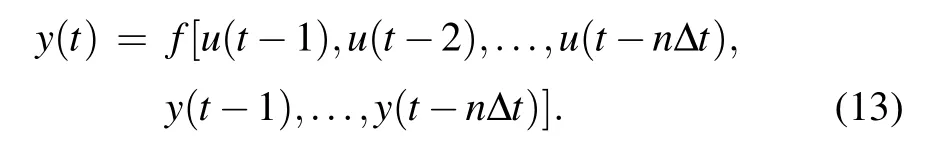
NARX neural networks show high performance in predicting the map based on the input and output of a dynamic system. The network model structure[49]is shown in Fig.12.Layer 1 represents the hidden layer,layer 2 represents the output layer,u(t) represents the input, and ˆyrepresents the output,f1andf2activation functions, IW is the input weight,LW is the output weight,b1is the bias of the first layer(input bias),b2is the bias of the second layer (output bias), andtis the time step. The input and output data will be multiplied by the corresponding weights through the delay line (TDLtapped delay line),and the offset is added,the excitation function is used to further establish the connection so that the previous value of the independent input signalu(t) and the next value of the dependent output signaly(t) can establish a regression time-series relationship,thereby building a complete cyclic dynamic network. The specific mathematical expression of the NARX network model is given as follows:

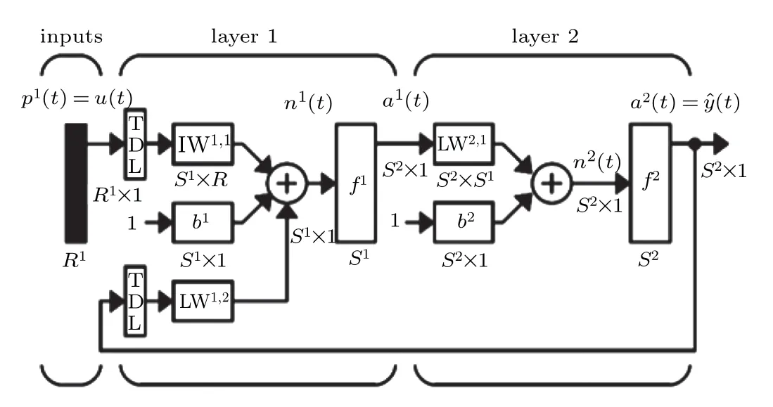
Fig.12. The structure diagram of the NARX neural network.

The NARX neural network model predicts the memristive map as shown in Fig.13.

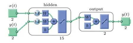
Fig.13. The NARX neural network model.

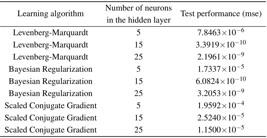
Table 2. The performance of the network with various learning algorithms and hidden layer neurons.

Fig. 14. Performance of the network: (a) means square error of test network,(b)error histograms.

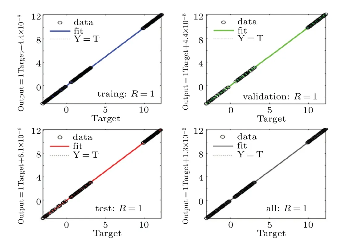
Fig.15. The correlation of target and output.

Fig. 16. The memristive map (2) with a = 3.00 for closed quasiperiodic, a=3.36 for chaos, a=3.40 for discrete periodic points and a=3.60 for hyperchaos: (a) phase trajectory of target attractors, (b)NARX neural network output.

The network model has two inputs (x,y) and two outputs (xˆ,yˆ). The data obtained by the map in the simulation results under the given system parameters and initial conditions, where the data set 36000 data are used for training(60% of the data set), 12000 data are used for validation(20% of the data set) and 12000 data are used for testing(20% of the data set). The training set is used for training to optimize the model iteratively, while the validation set further optimizes the model by adjusting hyperparameters. The test sets further monitor the model effect without participating in the training process. Training, testing, and verification data are performed randomly. Provide 20000 sets of data to the network for testing, the hidden layer uses hyperbolic tangent as the activation function, and the output layer uses a linear function as the activation function.The network training uses three different learning algorithms,namely Levenberg-Marquardt, Bayesian regularization, and quantized conjugate gradient.By selecting the number of neurons in the hidden layer with different numbers of neurons,the performance of the three different training algorithms is compared. Table 2 shows the performance(mean square error)of the network under different learning algorithms and different numbers of hidden layer neurons. It can be seen that using the Levenberg-Marquardt learning algorithm and 15 neurons in the hidden layer gives the best results. The performance(mean square error)and error histogram of the tested network are shown in Fig.14. As shown in Fig.15,the correlation between the output data and the target data is measured, whereR=1 indicates that the output and target are closely related.In the experimental simulation process,the obtained mean square error value is 2.1712×10−9. Therefore, the trained network can predict the map based on this mean square error value.

Table 3. Performance of the predicting of typical attractors.

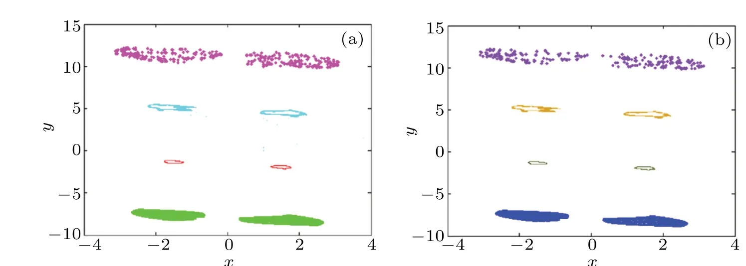
Fig.17. The memristive map(2)under different initial states: (a)phase trajectories of the target attractor,(b)NARX neural network output.

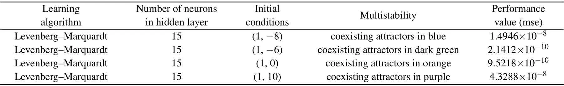
Table 4. Performance of the predicting of coexisting attractors.

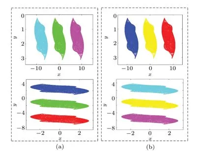
Fig.18. The memristive map(11)under the initial conditions(x0,y0)=(1−p, −2−q): (a)phase trajectories of target attractors,(b)output of NARX neural network prediction.

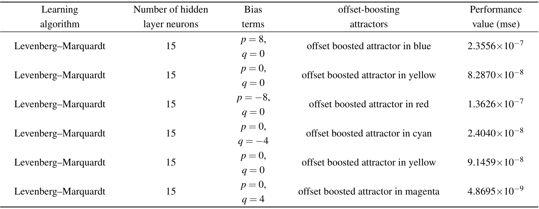
Table 5. Performance of the predicting of offset-boosting attractors.

Fig.19. The memristive map(12)with a=4.2 under the initial condition(x0,y0)=(1,−2): (a)phase trajectories of the target attractor with amplitude controlled,(b)NARX neural network prediction.

Table 6. Performance of the predicting of amplitude controlled attractors.

The algorithm is selected with the best training effect and the number of corresponding hidden layer neurons to predict the attractor phase trajectory of the map. Figure 16 gives the prediction comparison of the typical attractors’ phase trajectories; the multistability predictions are shown in Fig.17,the corresponding offset-boosting and amplitude modulation attractors’phase trajectories are shown in Figs.18 and 19. Tables 3-6 correspond to the predicted performance. Here, to better distinguish the phase trajectories,the real attractors(as the target)are marked in green and the predicted ones by the neural network are marked in red. From Figs. 16-19, the attractors’ phase trajectories are basically consistent with the corresponding NARX neural network prediction outputs, so the designed NARX neural network can successfully predict the hyperchaotic map.

7. Conclusion

When a discrete memristor and two trigonometric functions are applied in a discrete map, a novel map with coexisting chaos and hyperchaos is proposed, which also exhibits various regimes of multistability including the coexistence of quasi-periodic, chaotic, periodic, and hyperchaotic attractors.Numerical analysis shows that the emergence of multistability greatly depends on the initial conditions of the memristor.Furthermore,offset-boosting and amplitude control are discussed in detail by a linear transformation aiming at accelerating the application of chaotic sequences in radar and communication systems. The prediction based on NARX neural network verifies the consistency of numerical simulation and theoretical analysis. The application of memristive maps combined with image encryption algorithms[50-53]is expected soon.