GLOBAL STRONG SOLUTION AND EXPONENTIAL DECAY OF 3D NONHOMOGENEOUS ASYMMETRIC FLUID EQUATIONS WITH VACUUM∗
2021-10-28GuochunWU吴国春
Guochun WU(吴国春)
Fujian Province University Key Laboratory of Computational Science,School of Mathematical Sciences,Huaqiao University,Quanzhou 362021,China
E-mail:guochunwu@126.com
Xin ZHONG(钟新)†
School of Mathematics and Statistics,Southwest University,Chongqing 400715,China
E-mail:xzhong1014@amss.ac.cn
Abstract We prove the global existence and exponential decay of strong solutions to the three-dimensional nonhomogeneous asymmetric fluid equations with nonnegative density provided that the initial total energy is suitably small.Note that although the system degenerates near vacuum,there is no need to require compatibility conditions for the initial data via time-weighted techniques.
Key words nonhomogeneous asymmetric fluid equations;global strong solution;exponential decay;vacuum
1 Introduction
Asymmetric fluid equations,which were suggested and introduced by Eringen in the 1960s(see[18]),are a signi ficant step towards the generalization of the Navier-Stokes equations.They pertain to fluids which exhibit micro-rotational effects and micro-rotational inertia,and can be viewed as non-Newtonian.Physically,asymmetric fluid may represent fluids that consist of rigid,randomly oriented(or spherical particles)suspended in a viscous medium,where the deformation of fluid particles is ignored.It can describe many phenomena that appear in a number of complex fluids,such as suspensions,animal blood,and liquid crystals that cannot be characterized appropriately by the Navier-Stokes system,and as such they are important to scientists working on hydrodynamic-fluid problems.We refer the interested reader to the monograph[26],which provides a detailed derivation of the micropolar fluid equations from the general constitutive laws,together with an extensive review of the mathematical theory and applications of this particular model.
Let Ω⊆R3be a bounded smooth domain,we are concerned with the following threedimensional nonhomogeneous asymmetric fluid equations(see[26,pp.22–23]):

Here ρ,u,w,and P denote the density,velocity,micro-rotational velocity,and pressure of the fluid,respectively.The positive constantsµ1,ξ,µ2,and λ are the viscosity coefficients of the fluid.
We consider an initial boundary value problem for(1.1)with the initial condition

and the Dirichlet boundary condition

It should be noted that when there is no micro-structure(w=0 and ξ=0),the system(1.1)reverts to the classical nonhomogeneous Navier-Stokes equations,which have been studied by many researchers;please refer to[1,2,13–15,17,23,24,27–29]and references therein.
Let us turn our attention to the system(1.1).When the initial density is strictly away from vacuum(i.e.,ρ0is strictly positive),the authors[4]proved some existence and uniqueness results for strong solutions.Meanwhile,Braz e Silva et al.[5]investigated the global existence and uniqueness of solutions for the 3D Cauchy problem through a Lagrangian approach.On the other hand,when the initial density allows vacuum states,ukaszewicz[25](see also[26,Chapter 3])obtained the short-time existence of weak solutions provided that the initial functions u0and w0are inand the initial density ρ0is uniformly bounded and satis fieswhile Braz e Silva and Santos[12]established the global existence of weak solutions.In[9],under smallness assumptions on the initial data,weak solutions with improved regularity were obtained.At the same time,imposing a compatibility condition on the initial data,Zhang and Zhu[33]showed global existence of the unique strong solution with nonnegative density in R3under a smallness condition.Later on,Ye[32]improved their result by removing the compatibility condition and,furthermore,obtained the exponential decay of strong solutions.There are also other interesting studies on aspects of the nonhomogeneous asymmetric fluid equations,such as the vanishing viscosity problem[6,10],error estimates for the spectral semi-Galerkin approximations[16],the local existence of semi-strong solutions[7],and strong solutions in thin domains[8].In this paper,our purpose is to study the global existence and uniqueness of strong solutions of(1.1)–(1.3),and to describe the large time behavior of such strong solutions.The initial density is allowed to vanish.
Before stating our main result,we first explain the notations and conventions used throughout this paper.We write
For 1≤p≤∞and integer k≥0,the standard Sobolev spaces are denoted by

Our main results read as follows:
Theorem 1.1For constant q∈(3,6],assume that the initial data(ρ0≥0,u0,w0)satis fies

Let(ρ,u,w)be a strong solution to the problem(1.1)–(1.3).If T∗<∞is the maximal time of existence for that solution,then we have

where r and s satisfy

Remark 1.2The local existence of a unique strong solution with initial data as in Theorem 1.1 was established in[31].Hence,the maximal time T∗is well-de fined.
Remark 1.3It should be noted that(1.5)is independent of the micro-rotational velocity.The result indicates that the nature of the blowup for nonhomogeneous asymmetric fluid models is similar to the nonhomogeneous Navier-Stokes equations(see[22]),and does not depend on further sophistication of the equation(1.1)3.
We will prove Theorem 1.1 by contradiction in Section 3.In fact,the proof of the theorem is based on a priori estimates under the assumption that‖u‖Ls(0,T;Lr)is bounded independently of any T∈(0,T∗).The a priori estimates are then sufficient for us to apply the local existence result repeatedly to extend a local solution beyond the maximal time of existence T∗;this contradicts the maximality of T∗.
Based on Theorem 1.1,we can establish the global existence of strong solutions to(1.1)–(1.3)under some smallness condition.
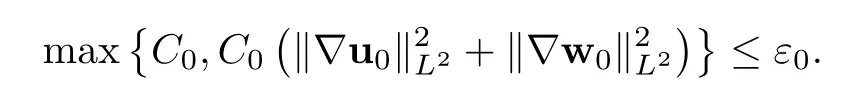
Theorem 1.4Let the conditions of Theorem 1.1 be in force.Then there exists a small positive constant ε0depending only on‖ρ0‖L∞,Ω,µ1,ξ,µ2,and λ such that,if

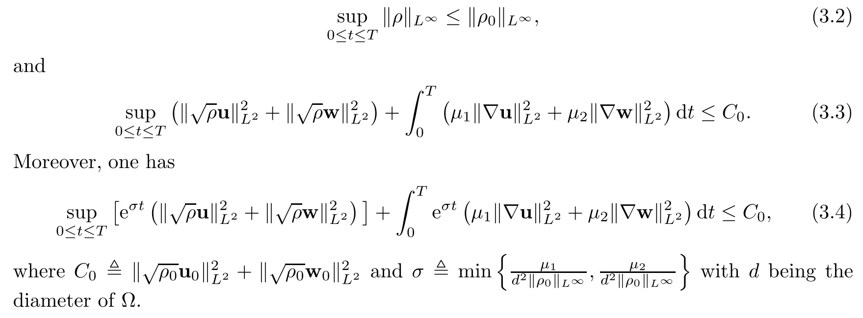
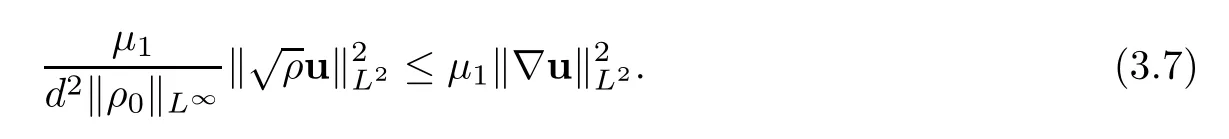
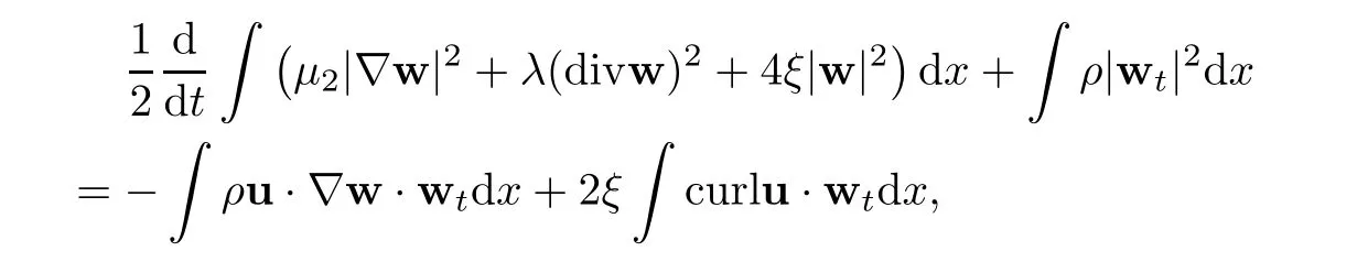
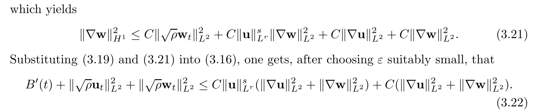
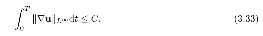
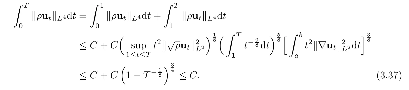
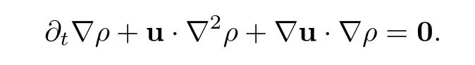
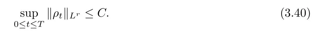
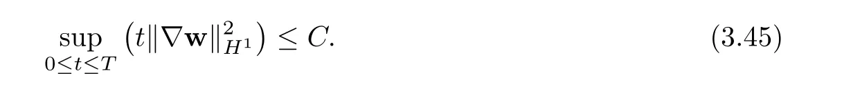
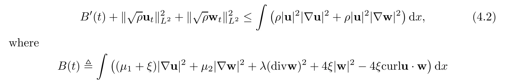
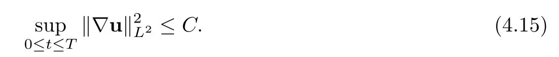
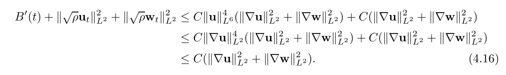
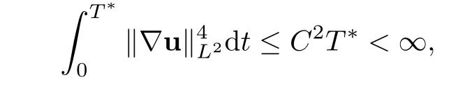
then the problem(1.1)–(1.3)has a unique global strong solution(ρ≥0,u,w)such that,for τ>0 and 2≤r Remark 1.6When there is no micro-structure(ξ=0 andw=0),Theorem 1.4 generalizes the previous result[15]for the 3D nonhomogeneous Navier-Stokes equations,which need some compatibility condition on the initial data andto be small.Furthermore,we get exponential decay rates of the solution rather than algebraic decay. The rest of this paper is organized as follows:in Section 2,we collect some elementary facts and inequalities that will be used later.Section 3 is devoted to the proof of Theorem 1.1.Finally,we give the proof of Theorem 1.4 in Section 4. In this section,we will recall some known facts and elementary inequalities which will be used frequently later. We start with the Gagliardo-Nirenberg inequality(see[20,Theorem 10.1,p.27]). Lemma 2.1(Gagliardo-Nirenberg)Let Ω⊂R3be a bounded smooth domain.Assume that 1≤q,r≤∞and j,m are arbitrary integers satisfying 0≤j The constant C depends only on m,j,q,r,a,and Ω.In particular,we have which will be used frequently in the next section. Next,we give some regularity properties(see[3,Proposition 4.3])for the following Stokes system: Lemma 2.2Suppose thatF∈Lr(Ω)with 1 Let(ρ,u,w)be a strong solution as described in Theorem 1.1.Suppose that(1.5)were false;that is,there exists a constant M0>0 such that Lemma 3.1It holds that Proof1.The desired(3.2)follows from(1.1)1and divu=0(see[24,Theorem 2.1]).Moreover,from(1.1)1and ρ0≥0,we have ρ(x,t)≥0. 2.Multiplying(1.1)2byu,(1.1)3byw,and integrating by parts,we obtain that Integrating(3.5)over[0,T]leads to(3.3). 3.From(3.2)and the Poincar´e inequality(see[30,(A.3),p.266]) with d being the diameter of Ω,we arrive at Hence,we get Similarly,we have which,together with Gronwall’s inequality,leads to(3.4),and completes the proof of Lemma 3.1. Lemma 3.2Under the condition(3.1),there exists a positive constant C depending only on M0,Ω,µ1,µ2,ξ,λ,and the initial data such that,for i∈{0,1,2}, Proof1.Multiplying(1.1)2byutand integrating by parts yields Multiplying(1.1)3bywtand integrating by parts leads to which,combined with(3.10),leads to Integrating(3.22)over[0,T],together with(3.1),(3.3),and(3.12),leads to(3.9)with i=0.For i∈{1,2},we can obtain similar results. Lemma 3.3Under the condition(3.1),there exists a positive constant C depending only on M0,Ω,µ1,µ2,ξ,λ,and the initial data such that,for i∈{1,2}, Multiplying(3.24)byut,(3.25)bywt,and integrating the resulting equality by parts over Ωand summing it,we obtain that Consequently,we derive(3.23)from(3.31),Gronwall’s inequality,(3.9),(3.32),and(3.4). Lemma 3.4Under the condition(3.1),there exists a positive constant C depending only on M0,Ω,µ1,µ2,ξ,λ,and the initial data such that Proof1.We obtain from Lemma 2.2,Sobolev’s inequality,the Gagliardo-Nirenberg inequality,(3.2),(3.19),(3.21),(3.9),and Young’s inequality that,for σ being as in Lemma 3.1, This,combined with Sobolev’s embedding theorem,(3.9),(3.1),(3.3),and(3.4),implies that 2.By H¨older’s inequality,Sobolev’s inequality,and(3.2),we have which,together with H¨older’s inequality,implies for any 0≤a As a consequence,if T≤1,we obtain from(3.35),H¨older’s inequality,and(3.23)that If T>1,one deduces from(3.36),(3.35),H¨older’s inequality,and(3.23)that Hence,we infer from(3.36)and(3.37)that This combined with(3.34)leads to(3.33). Lemma 3.5Let q be as in Theorem 1.1.Then there exists a positive constant C depending only on M0,Ω,µ1,µ2,ξ,λ,q,and the initial data such that,for r∈[2,q), ProofTaking the spatial derivative∇on the transport equation(1.1)1together with(1.1)4leads to Thus,standard energy methods yield for any q∈(2,∞)that which combined with Gronwall’s inequality and(3.33)gives that Notice that we have This,together with(3.39)and(3.9),yields Thus,(3.38)follows from(3.2),(3.39),and(3.40). Lemma 3.6Let q be as in Theorem 1.1,there exists a positive constant C depending only on M0,Ω,µ1,µ2,ξ,λ,q,and the initial data such that Proof1.We obtain from(3.18),(3.2),Sobolev’s inequality,and(3.9)that which together with(3.23)and(3.9)yields that From(3.20),(3.2),Sobolev’s inequality,and(3.9),one has which combined with(3.23)and(3.9)yields 2.We get from(3.17),(3.2),(3.39),Sobolev’s inequality,(3.42),and(3.44)that which,together with(3.9),(3.4),(3.23),and(3.43),implies that Similarly,one can deduce that Hence,(3.41)follows from(3.43)and(3.45)–(3.47). With Lemmas 3.1–3.6 in hand,we are now in a position to prove Theorem 1.1. Proof of Theorem 1.1We argue by contradiction.Suppose that(1.5)were false;that is,that(3.1)holds.Note that the general constant C in Lemmas 3.1–3.6 is independent of t satis fies the initial condition(1.4)at t=T∗.Therefore,taking(ρ,u,w)(x,T∗)as the initial data,one can extend the local strong solution beyond T∗,which contradicts the maximality of T∗.Thus we finish the proof of Theorem 1.1. Throughout this section,we denote that Note that Lemma 3.1 also holds true,due to its independence from the condition(3.1). Lemma 4.1Let(ρ,u,w)be a strong solution to the system(1.1)–(1.3)on(0,T).Then there exist positive constants C and L depending only on‖ρ0‖L∞,Ω,µ1,µ2,λ,and ξ such that,for any t∈(0,T), whereµ≜µ1+µ2+λ+2ξ+8ξd2. Proof1.We obtain from(3.11)and the Cauchy-Schwarz inequality that which yields that which combined with(4.8)implies(4.1)and finishes the proof of the lemma. Lemma 4.2Let(ρ,u,w)be a strong solution to the system(1.1)–(1.3)on(0,T)and letµbe as in Lemma 4.1.Then there exists a positive constant ε0depending only on‖ρ0‖L∞,Ω,µ1,µ2,λ,and ξ such that where L is the same as in(4.1).In view of the regularities ofuandw,one can obtain that both E(t)and Φ(t)are continuous functions on(0,T).By(4.1),there is a positive constant M depending only on‖ρ0‖L∞,Ω,µ1,µ2,λ,and ξ such that Otherwise,by the continuity and monotonicity of Φ(t),there is a T0∈(0,T]such that On account of(4.13),it follows from(4.12)that Recalling the de finitions of E(t)and Φ(t),we deduce from the above inequality that By virtue of the claim we showed in the above,we derive from(4.12)that provided that(4.11)holds true.This implies(4.10)and consequently completes the proof of Lemma 4.2. Lemma 4.3Let(4.11)be in force and let σ be as in Theorem 1.4.Then for ζ(T)≜min{1,T},there exists a positive constant C depending only on Ω,µ1,ξ,µ2,λ,q,and the initial data such that Proof1.We obtain from Lemma 4.2 that Choosing s=4 and r=6 in(3.22),together with Sobolev’s inequality and(4.15),yields that Then we deduce from(4.16)multiplied by eσt,Gronwall’s inequality,(3.12),and(3.4)that 2.Choosing s=4 and r=6 in(3.30),together with Sobolev’s inequality and(4.15),leads to Multiplying(4.18)by eσtgives rise to which,combined with Gronwall’s inequality,(4.17),and(3.4),implies that for ζ(T)≜min{1,T}, 3.Choosing s=4 and r=6 in(3.19)and(3.21),together with Sobolev’s inequality and(4.15),yields that This along with(4.19)and(4.17)indicates that Hence,(4.14)follows from(4.19)and(4.20). Now,we can give the proof of Theorem 1.4. Proof of Theorem 1.4Let ε0be the constant stated in Lemma 4.2,and suppose that the initial data(ρ0,u0,w0)satis fies(1.4)and According to[31],there is a unique local strong solution(ρ,u,w)to the system(1.1)–(1.3).Let T∗be the maximal existence time to the solution.We will show that T∗=∞.Suppose,by contradiction,that T∗<∞.Then,by(1.5),we deduce that for(s,r)=(4,6), which combined with the Sobolev inequality‖u‖L6≤C‖∇u‖L2leads to By Lemma 4.2,for any 0 which implies that which is in contradiction to(4.21).This contradiction provides us with the fact that T∗=∞,and thus we obtain the global strong solution.Moreover,the exponential decay rate(1.9)follows from(4.14).This finishes the proof of Theorem 1.4.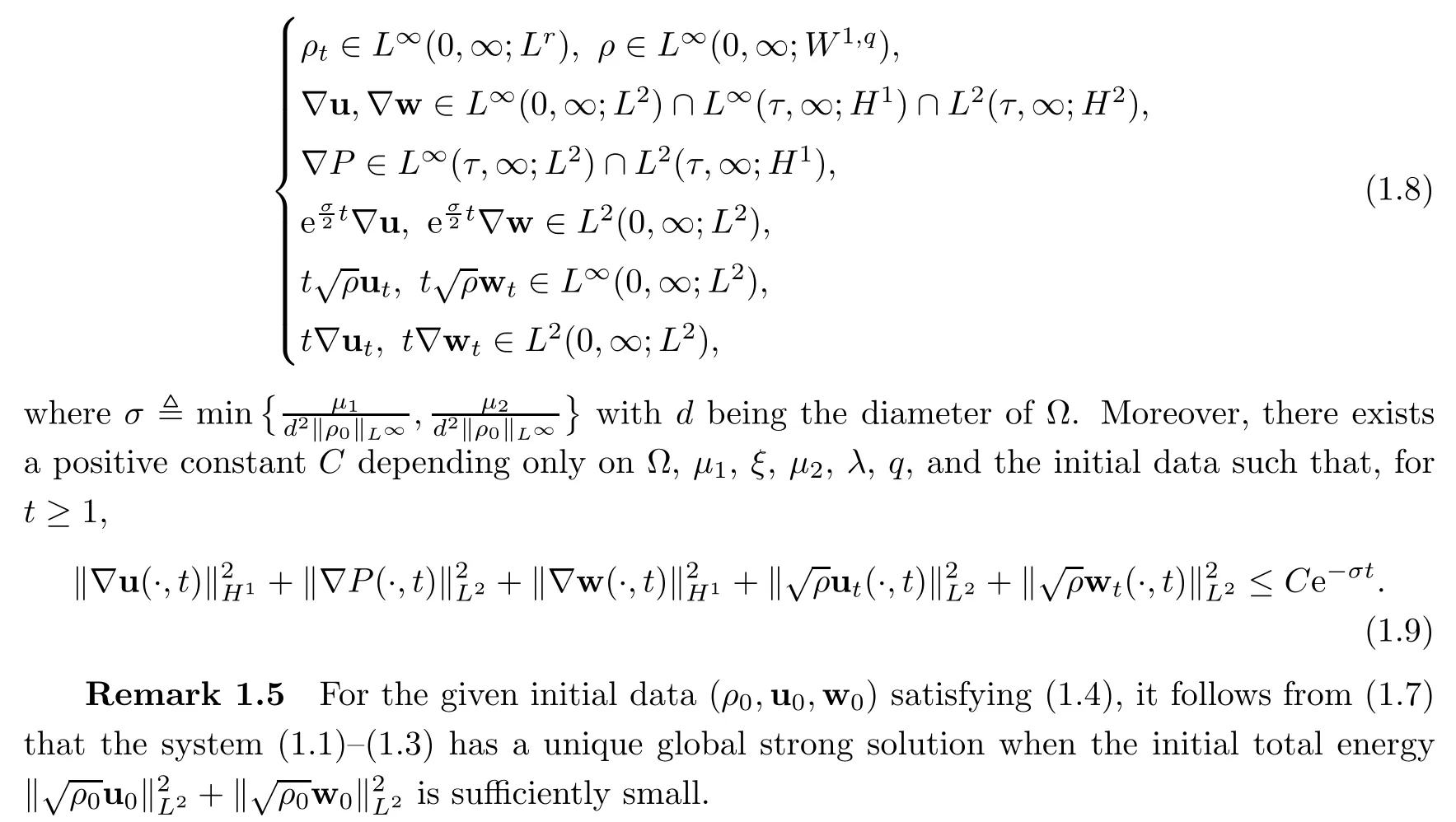
2 Preliminary


3 Proof of Theorem 1.1


4 Proof of Theorem 1.4


猜你喜欢
杂志排行

Acta Mathematica Scientia(English Series)的其它文章
- RIGIDITY RESULTS FOR SELF-SHRINKING SURFACES IN R4∗
- CONTINUOUS TIME MIXED STATE BRANCHING PROCESSES AND STOCHASTIC EQUATIONS∗
- SOME OSCILLATION CRITERIA FOR A CLASS OF HIGHER ORDER NONLINEAR DYNAMIC EQUATIONS WITH A DELAY ARGUMENT ON TIME SCALES∗
- COARSE ISOMETRIES BETWEEN FINITE DIMENSIONAL BANACH SPACES∗
- ZERO KINEMATIC VISCOSITY-MAGNETIC DIFFUSION LIMIT OF THE INCOMPRESSIBLE VISCOUS MAGNETOHYDRODYNAMIC EQUATIONS WITH NAVIER BOUNDARY CONDITIONS∗
- THE PRECISE NORM OF A CLASS OF FORELLI-RUDIN TYPE OPERATORS ON THE SIEGEL UPPER HALF SPACE∗