Lina Wu,Qing Gao,Yungui Gong,Yiding Jiaand Tianjun Li

1 School of Sciences,Xi’an Technological University,Xi’an 710021,China

2 School of Physical Science and Technology,Southwest University,Chongqing 400715,China

3 School of Physics,Huazhong University of Science and Technology,Wuhan,Hubei 430074,China

4 CAS Key Laboratory of Theoretical Physics,Institute of Theoretical Physics,Chinese Academy of Sciences,Beijing 100190,China

5 School of Physical Sciences,University of Chinese Academy of Sciences,Beijing 100049,China

Abstract We consider the polynomial inflation with the tensor-to-scalar ratio as large as possible which can be consistent with the quantum gravity(QG)corrections and effective field theory(EFT).To get a minimal field excursionΔφ for enough e-folding number N,the inflaton field traverses an extremely flat part of the scalar potential,which results in the Lyth bound to be violated.We get a CMB signal consistent with Planck data by numerically computing the equation of motion for inflaton φ and using Mukhanov–Sasaki formalism for primordial spectrum.Inflation ends at Hubble slow-roll parameter=1or=0.Interestingly,we find an excellent practical bound on the inflaton excursion in the format a +b,where a is a tiny real number and b is at the order 1.To be consistent with QG/EFT and suppress the high-dimensional operators,we show that the concrete condition on inflaton excursion isFor ns=0.9649,Ne=55,andwe predict that the tensor-to-scalar ratio is smaller than 0.0012 for such polynomial inflation to be consistent with QG/EFT.

Keywords:polynomail inflation,Lyth bound,tensor-to-scalar ratio

1.Introduction

Inflation provides a natural solution to the well-known flatness,horizon,and monopole problems,etc,in the standard big bang cosmology[1–4].And the observed temperature fluctuations in the cosmic microwave background radiation(CMB)strongly indicates an accelerated expansion at a very early stage of our Universe evolution,i.e.inflation.In addition,the inflationary models predict the cosmological perturbations for the matter density and spatial curvature due to the vacuum fluctuations of the inflaton,and thus can explain the primordial power spectrum elegantly.Besides the scalar perturbation,the tensor perturbation is also generated.Especially,it has special features in the B-mode of the CMB polarization data as a signature of the primordial inflation.

The Planck satellite measured the CMB temperature anisotropy with an unprecedented accuracy.From the latest observational data[5,6],the scalar spectral index ns,the running of the scalar spectral indexthe tensor-to-scalar ratio r,and the scalar amplitude Asfor the power spectrum of the curvature perturbations are respectively constrained to be

There is no sign of primordial non-Gaussianity in the CMB fluctuations.On the other hand,from the analysis of BICEP2/Keck CMB polarization experiments[7,8],the upper limits are set to r<0.07 at 95%CL.The future QUBIC experiment[9,10]targets to constrain the tensor-to-scalar ratio of 0.01 at 95% CL with two years of data.Therefore,the interesting question is how to construct the inflation models which can be consistent with the Planck results and have large tensor-to-scalar ratio.The energy scale of inflation is described by the ratio between the amplitude of the tensor mode and scalar mode of CMB[11]

The inflationary models with r～0.01 are very interesting for two reasons:(1)from the above equation(2),the energy scale of inflation is close to the unification scale in the grand unified theory(GUT),which is around 2×1016GeV;(2)they might be probed by the future experiments.On the other hand,the naive analysis of the Lyth bound gives[12,13],where N is the number of e-folding,and MPlis the reduced Planck scale,i.e.Thus,the infalton excursionΔφ is larger than about 2MPlfor r=0.01 and N～55.And we will define the large tensor-to-scalar ratio as r>0.01,and call it the large field inflation ifΔφ>2MPl.Therefore,if the Lyth bound is valid,the big challenge to the inflationary models with large r is the high-dimensional operators in the inflaton potential from the effective field theory(EFT)point of view,which may be generated by the quantum gravity(QG)effects,since such highdimensional operators can not be suppressed by MPland then are out of control.Three kinds of solutions to this the problem are:(1)The natural inflation since the QG corrections may be forbidden by the discrete symmetry[14,15].However,the QG does not preserve the global symmetry.(2)The phase inflation since the phase of a complex field may not play an important role in the non-renormalizable operators from QG effects[16–18].(3)The polynomial inflation with the Lyth bound violation and smallΔφ[19–32].However,no one has constructed a concrete,solid,and interesting infaltionary model withΔφ≤O(0.1)MPlfor the whole e-folding stretch.And also,the Gao–Gong–Li bound on inflaton excursion[23]isΔφ<0.1 MPlwith a modified tensor-toscalar bound r<0.02.It’s too low and can not be saturated,and it is not clear whether there exists a new practical bound.Note that,the minimal field excursionΔφ plays an important role to determine the upper bound of r.

ForΔφ<0.1 MPl,we can expand the generic inflaton potential via the Taylor series.Thus,for simplicity,we shall study the polynomial inflation with the tensor-to-scalar ratio as large as possible which is consistent with the QG corrections and EFT.We do realize the small field inflation with a large r,and then the Lyth bound is violated obviously.Interestingly,we find an excellent practical bound on the

inflaton excursion in the formatwhere a is a small real number and b is at the order 1.To be consistent with QG/EFT and suppress the high-dimensional operators,we show that the concrete condition on inflaton excursion is0.632.For ns=0.9649,Ne=55,andwe predict that the tensor-to-scalar ratio is smaller than 0.0012 for such polynomial inflation to be consistent with QG/EFT.The interesting question is whether our polynomial inflation can arise from a concise function or a more complete theory.From our study during the last seven years,we have not found it yet.

2.The polynomial inflation

We will consider the order 5 polynomial inflation for numerical study,i.e.

The slow-roll parameters∊,η,and ξ2are defined as

The number of e-folding before the end of inflation is

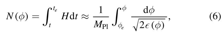
where the inflaton value φeat the end of inflation is determined by=̈0or∊=1,where a is the scale factor.If∊(φ)is a monotonic function during inflation,we have∊(φ)>∊(φ*)=∊=r/16,and then get the Lyth bound[12]

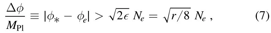
where the subscript‘*’means the value at the horizon crossing,and ns,αsand r are evaluated at φ*.For example,the Lyth bound givesΔφ=1.947MPlfor r=0.01 and Ne=55.Thus,to realize the small field inflation with large r,the Lyth bound must be violated.In other words,∊(φ)should not be a monotonic function and has at least one minimum between φ*and φe[19].

2.1.Numerical results

To compute observable quantities for the CMB,we numerically evolve the scalar field according to the Friedman equation and equation of motion for φ:

For numerical purposes it is more convenient to rewrite the inflaton evolution as a function of conformal time τ rather than time t.Usingthe cosmological evolution equation becomes

For convenience,we use the slow-roll parameters defined via Hubble parameter:

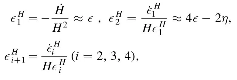
where dots denote derivatives respect to the cosmic time.The inflation ends ator=1.

To get the minimal field excursionΔφ and enough e-folding number N for each r,the inflaton field must traverse an extremely flat part of the scalar potential.This is similar to ultra-slow-roll inflation(USR)[34–38].There are 3 inflection points for the 5th degree polynomial.We find a set of parameters which make sure there is an inflection point φinflduring inflation and the derivative of V(φ)at the inflection point should be small,i.e.

In such situation,an exact scalar spectral index nsand tensorto-scalar ratio r will numerically calculated by primordial spectrum using the Mukhanov–Sasaki formalism[39,40].The scalar modeuk=-zR and tensor mode vkof primordial perturbation are given by

whereR is the comoving curvature perturbation,andIn the limit k→∞,the modes are in the Bunch–Davies vacuumandThe scalar and tensor spectrum of primordial perturbations at CMB scales can be accurately expressed as

Then the spectral index,running of the spectral index and tensor-to-scalar ratio at k*=aH=0.05 MPc-1can determined by

To simplify the numerical study,we choose Ne=55,as well as the best fit for nsand αs,i.e.ns=0.9649,αs=-0.0045 and As=2.20×10-9[7,8].Without loss of generality,we will take φ*=0.r andΔφ for the 5th degree polynomial inflation are given in figure 1,where the red point-line is corresponding to the low bound on inflaton excursion.The inflation ends ator=0.

Figure 1.r versusΔφ for the polynomial inflation.Here the e-folding number,the scalar spectral index and the relative running are fixed to be N=55,ns=0.9649,and αs=-0.0045,respectively.The red line corresponds to the the low bound on the inflaton excursion.The three horizontal dashed lines correspond to Δφ=0.632,1.0,2.0 MPl,respectively.

To be concrete,we present some examples.Taking several tensor-to-scalar ratios r=0.01–0.056,we try our best to get the minimal inflation excursions numerically.Using the relation of the CMB observations to the potential parameters at the beginning of inflation,which will be shown in equation(18),we first obtain the values of parameters λ1,2,3and V0.Then the last two parameters λ4and λ5can numerically acquired by solving the equation(10)and requiring that there be at least one inflection point during inflation.In this way,we get an USR inflationary model6This feature can ensure the formation of primordial black holes which deserves further study.with a smaller field excursion since the inflaton slows down around the inflection point.The results are shown in table 1.To understand why our polynomial potential violates the Lyth bound but is consistent with the Planck results,we plot the hubble slowroll parametersandin figure 2 for the model with r=0.01.The potential V/V0and its first derivativewiththeparametersλi=(-3.6188×10-2,-10.0437×10-3,-9.8543×10-3,32.1351×10-2,-35.5515×10-2)are shown in figure 3.There is an inflection point φinfl=0.515 MPl,andis close to zero.The evolution of inflaton is extremely slow around φinfland the slow-roll parametersdecreases several orders of magnitude at φinfl.

2.2.Slow roll approximation

In the slow-roll inflation with inflaton potential V(φ),the observations are

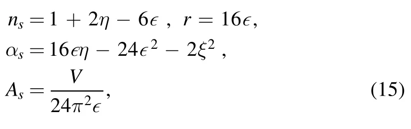
Since the inflation potential has order 5 polynomial,we need take into account the higher order corrections for nsand r.Thehigher order corrections[33,41–43]are given in

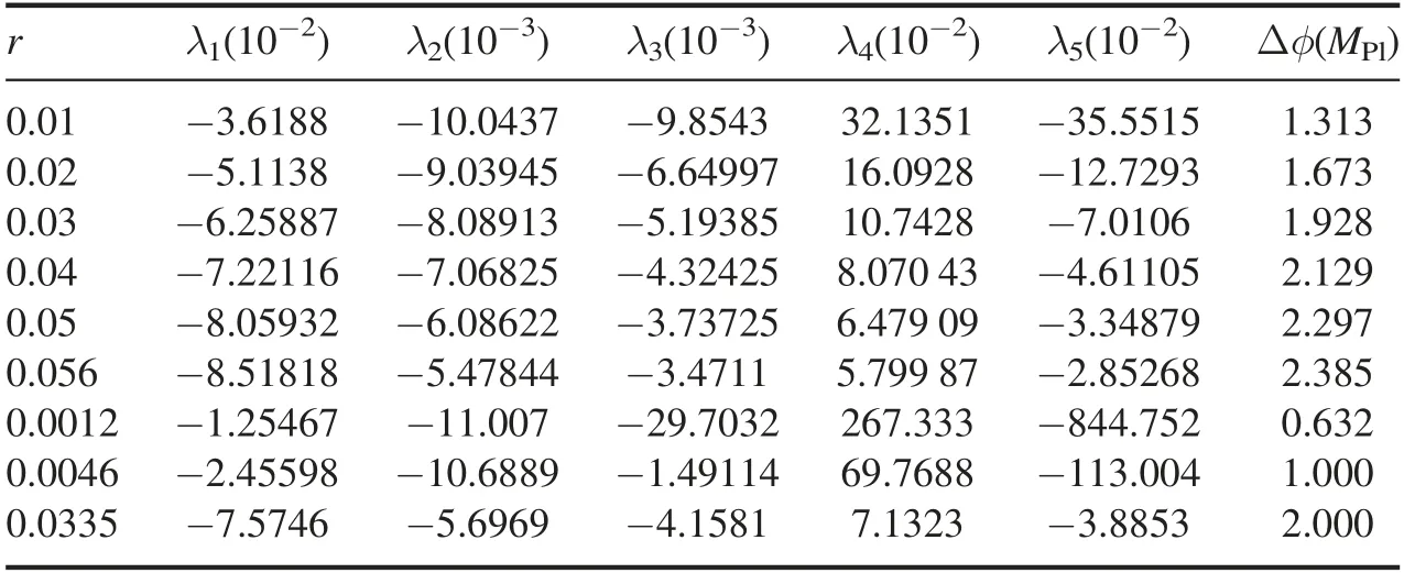
Table 1.The low bound of inflaton excursion and the parameters for inflation potential.Here e-folding number,the scalar spectral index and the relative running are fixed to the central value,i.e.N=55,ns=0.9649,and αs=-0.0045.

Figure 2.The evolution of Hubble flow slow-roll parameters(blue solid line)and(red dashed line).

whereC=-2 +ln 2+γ≃-0.7296with γ the Euler–Mascheroni constant.The slow-roll parameters at the horizon crossing φ*=0 are approximated as

Then,the parameters V0and λ1,2,3can be determined by the observations in equation(15)as follows:

Therefore,we can get the higher order corrections of these observations

Solving these equations with αs=-0.0045,we find that the second-order corrections will give a tiny contribution Δr<-1.5×10-3for r<0.056 andΔns～4.9×10-3for ns=0.9649.These corrections for CMB are still within 2 σ range of Planck data.

2.3.The lower bound on inflaton excursion

For slow-roll inflation,we obtainif∊(φ)is a constant during inflation.However,in general,∊(φ)is a φ dependent varying function during inflation.Interestingly,for the slow-roll inflation with polynomial inflaton potential,we find that the generic lower bound on inflaton excursion is a linear function ofi.e.approximately.The results for a fixed αs=-0.0042 and N=55 are show in figure 4.The black line in figure 4(a)is the fitted linear equation 0.4569 +8.2247for fixed ns=0.9649.We also check the field excursion variation as nsincreases.The different color points in figure 4 are corresponding to different central value of ns.For the variation of ns,the low bound ofΔφ is pushed toward to a smaller value,which is consistent with previous results[28].On the other hand,after fixing the tensor-to-scalar ratio r=0.01,we compare the field excursion results from equation(8)and slow-roll approximation in equation(16)for ns=0.9625,0.9655,0.9685.The results are concluded in table 2.We can find that the field excursion become smaller at order 10-3as nsincreases.

2.4.The consistency with QG and EFT

To be consistent with QG/EFT and suppress the highdimensional operators,we require thatshould be at the order of 0.1,i.e.★7Here,we want the higher order coefficient to be one order of magnitude smaller than the lower order coefficient in the Taylor expansion..To minimize the absolute value ofwe can chooseand thenThus,to be consistent with QG and EFT,we require0.632≃.

Table 2.The low bound of inflaton excursion.Δφ is numerically calculated from equation(8),and δφ is calculated with high order corrections under the slow roll approximation.Here the tensor-toscalar ratio is fixed to be r=0.01.

With QG/EFT effects,inflation excursions are smaller thanΔφ<0.632MPl.We predict that the upper bound on tensor-to-scalar ratio r for single field slow-roll inflation is r≤0.0012.The corresponding parameters are also shown in table 1.Meanwhile,for the inflaton excursionsΔφ～1MPlandΔφ～2MPl,we find that the maximal tensor-to-scalar ratios are r～0.0046 and r～0.0335,respectively for Ne=55.While the Lyth bound gives r～0.0026 and r～0.0106,respectively.Thus,the Lyth bound is indeed violated in our polynomial inflation.Our results are consistent with the current cosmological observation data and might be probed by the future observed results of CMB polarization missions[44–49]and gravitational waves experiments[50],which will detect the tensor-to-scalar ratio at the order of 10-3.

3.Conclusions

We have considered the polynomial inflation with the tensorto-scalar ratio as large as possible which is consistent with the QG corrections and EFT.We got the small field inflation with large r,and then the Lyth bound is violated obviously,since the evolution of the slow-roll parameters are very slow and the inflation enters USR around the inflection point.Interestingly,we found an excellent practical bound on the inflaton excursion in the formatwhere a is a small real number and b is at the order 1.To be consistent with QG/EFT and suppress the high-dimensional operators,we show that the concrete condition on inflaton excursion is0.632≃.For ns=0.9649,Ne=55,andwe predict that the tensor-to-scalar ratio is smaller than 0.0012 for such polynomial inflation to be consistent with QG/EFT.

Acknowledgments

This work was supported in part by the Projects 11875062,11875136,and 11947302 supported by the National Natural Science Foundation of China,by the Major Program of the National Natural Science Foundation of China under Grant No.11690021,by the Key Research Program of Frontier Science,CAS.This work was also supported in part by the Program 2020JQ-804 supported by Natural Science Basic Research Plan in Shanxi Province of China,and by the Program 20JK0685 funded by Shanxi Provincial Education Department.