Yangli XU (徐仰丽), Liuwei MENG (孟留伟), Xiaojing CHEN (陈孝敬),Xi CHEN(陈熙),Laijin SU(苏来金),Leiming YUAN(袁雷明),Wen SHI(石文) and Guangzao HUANG (黄光造)

1 Wenzhou Vocational College of Science and Technology,Wenzhou 325006,People’s Republic of China

2 College of Electrical and Electronic Engineering, Wenzhou University, Wenzhou 325035, People’s Republic of China

3 Research and Development Department,Hangzhou Goodhere Biotechnology Co.Ltd,Hangzhou 311100,People’s Republic of China

4 College of Life and Environmental Science,Wenzhou University,Wenzhou 325035,People’s Republic of China

Abstract Tegillarca granosa, as a popular seafood among consumers, is easily susceptible to pollution from heavy metals.Thus, it is essential to develop a rapid detection method for Tegillarca granosa.For this issue, five categories of Tegillarca granosa samples consisting of a healthy group;Zn,Pb,and Cd polluted groups;and a mixed pollution group of all three metals were used to detect heavy metal pollution by combining laser-induced breakdown spectrometry(LIBS)and the newly proposed linear regression classification-sum of rank difference (LRC-SRD)algorithm.As the comparison models, least regression classification (LRC), support vector machine (SVM), and k-nearest neighbor (KNN) and linear discriminant analysis were also utilized.Satisfactory accuracy (0.93) was obtained by LRC-SRD model and which performs better than other models.This demonstrated that LIBS coupled with LRC-SRD is an efficient framework for Tegillarca granosa heavy metal detection and provides an alternative to replace traditional methods.

Keywords: Tegillarca granosa, sum of ranking difference, heavy metal, linear regression classification

1.Introduction

Due to the rapid development of national industrialization and the low public awareness of environmental protection,a large amount of domestic garbage and industrial wastes containing toxic heavy metals are discharged into rivers, lakes and seas[1].As a result,serious pollution of water and shellfish poses a threat to human health when the toxic heavy metal elements ascend the food chain and enter the human body.Tegillarca granosa, which is well known as blood cockle, is one of the most popular seafoods among consumers because of its delicious taste and rich nutrition [2].As a kind of seafood with low activity, filter-feeding habits and wide distribution,Tegillarca granosais very likely to be exposed to environmental heavy metal pollution.Moreover,Tegillarca granosais also vulnerable to heavy metal absorption and easily suffers from heavy metal pollutant accumulationin vivo[3].According to the related literature, eating heavy metal polluted seafood will lead to enzyme inactivation in the body and increase the risk of chronic poisoning [4].Moreover, heavy metal pollution has become one of the most dangerous factors ofTegillarca granosabreeding.To ensure the quality and safety ofTegillarca granosaand prevent heavy metals polluted seafood from entering the consumer market,developing a rapid detection technology is necessary for identifyingTegillarca granosacontaminated with heavy metals.This is of great significance for improving the economic benefits of seafood farmers and ensuring the health and safety of consumers.

For the detection of heavy metals, the commonly used method is the traditional wet chemical method coupled with expensive analytical equipment, such as inductively coupled plasma mass spectrometry (ICP-MS) [5], atomic absorption spectrometry [6] and ICP optical emission spectrometry [7].Complex sample preparations, time-consuming process and the use of toxic and dangerous chemicals in detection means that these instrumental methods cannot meet the needs of fast,non-destructive or micro-destructive testing, although highly accurate and sensitive detection results can be acquired[8].In contrast,spectral technology has become of interest due to its green, fast and accurate characteristics.Among the spectral technologies, laser-induced breakdown spectroscopy (LIBS)as a kind of atomic emission spectroscopy technique is a good candidate for the detection of heavy metals and can detect any heavy metals regardless of the sample’s physical states.The main process of LIBS is to ablate a sample by a high-power laser pulse to generate a high-temperature plasma.Shortly afterward, emission lines of the target sample are emitted from the cooling plasma and are collected by a spectrometer[9].Because of the one-to-one correspondence relationship between the target elements and the emission lines of spectra,quantitative and qualitative analyses of target elements can be performed without a laborious and time-consuming sample pretreatment process[10].Moreover,many commercial LIBS devices have been developed and applied widely to replace many traditional methods for elemental detection.According to the related studies, LIBS has applied in environmental monitoring [11], food safety [12], the fuel industry [13] and space exploration [14].In this study, LIBS will be implemented to rapidly detect the heavy metal pollution inTegillarca granosa.

In ideal situations,specific emission lines would be used to establish the detection model of heavy metals after the collection of LIBS data.However,it is difficult to directly use univariate models for heavy metal detection because of the matrix effect of the target sample, self-absorption of plasma and interference and synergy between excitation lines[15,16].On the other hand,some elements’specific emission lines may overlap due to the mutual interferences of different components in the sample.Moreover, some of the emission lines of certain target elements in the sample cannot even be excited.As a result, the intensity or position of the emission lines of an analyte cannot be used as a basis for establishing qualitative and quantitative models.To fully use LIBS data and build a suitable detection model, multivariate calibration models, such as linear discriminant analysis (LDA), support vector machine (SVM), and k-nearest neighbor (KNN), are usually recommended to construct the classification or regression model [17,18].Good prediction results have been obtained by implementing these methods.Nevertheless,there are still two issues to be solved for the analysis of LIBS data.The above-mentioned calibration methods are usually used to process relatively low-dimensional data (dozens to thousands of variables) to establish a calibration model and have been used in several spectral analysis[19–21].However,LIBS data have more than tens of thousands of variables.Thus, a suitable algorithm is needed for this kind of high-dimensional data.To address this problem, least regression classification(LRC) [22] as a nonparametric and powerful algorithm, was adopted as the classifier to detect heavy metals inTegillarca granosa.In addition, the accuracy of the classifier is another issue in the detection of heavy metals inTegillarca granosa.To further improve LRC classifier’s performance, it is recommended to use a consensus model by combining several sub-models.For accurate performance, the sum of ranking differences(SRD)algorithm was used and combined with the LRC algorithm to create the LRC-SRD classification model.SRD is a comparison algorithm for models and methods that does not consider the data scale [23].The main calculation process was as follows: first, LIBS data containing tens of thousands of variables were divided into several segments evenly(the optimal segments could be obtained by comparing the performance of model in different segments);then,several LRC classification models (the number of models was equal to the number of segments) were established based on the divided segments and four instance values for each sample were obtained from an LRC classifier.Finally, the prediction result for each sample was regarded as the input matrix of SRD to calculate the SRD value for each LRC model and identify the classes of target samples.Similarly,the categories of all samples are determined according to the LRC-SRD algorithm.To the best of our knowledge,this is the first study to propose the LRC-SRD algorithm for qualitatively assessing heavy metal pollution.

To evaluate the ability of combining the LRC-SRD algorithm and LIBS technology to rapidly determine the heavy metal pollution ofTegillarca granosa, this study designed an experiment in whichTegillarca granosawas manually cultivated and contaminated with cadmium (Cd),zinc(Zn),lead(Pb)and their mixture for 10 d.In contrary,the uncontaminated sample group was also cultivated at the same time.As a result, 150 sample pellets that evenly came from five groups were prepared to collect LIBS data and develop LDA, SVM, KNN, LRC and LRC-SRD classifiers.Then the performance of these classifiers was compared, and the feasibility of rapidly determining heavy metals inTegillarca granosaby the newly proposed LRC-SRD method was also evaluated.In short, the objects of this study were as follows:(1) obtaining heavy metal-contaminated samples and healthy samples; (2) collecting LIBS data ofTegillarca granosasamples; (3) reconstructing LDA, SVM, KNN, LRC and LRC-SRD classifiers and comparing the performances of these classification models;and(4)assessing the feasibility of determining heavy metal contamination inTegillarca granosasamples by combining LIBS technology and the LRC-SRD algorithm.

2.Material and methods

2.1.Sample preparation

Tegillarca granosasamples were cultured by imitating their natural growth environment.Specifically,Tegillarca granosasamples were firstly divided into five groups,namely,control group(healthy),lead-zinc-cadmium(Pb–Zn–Cd)mixed stress group,lead(Pb)stress group,cadmium(Cd)stress group and zinc (Zn) stress group.During the farming ofTegillarca granosa, the heavy metal elements Pb, Cd and Zn from PbCH3COO·3H2O(1.833 mg l−1),CdCl2(1.634 mg l−1),and ZnSO4·7H2O(4.424 mg l−1)(these chemicals were purchased from National Standards Material Network-Beijing Century Aoke Biotechnology Co.Ltd, Beijing City, China) were dissolved in the cultivation water.The mixed stress group ofTegillarca granosawas exposed to a mixture heavy metal solution of above the three chemicals.In contrast,the control group was cultured with seawater under the same conditions without heavy metal addition.Notably, the concentrations of several heavy metal were prepared on basis of the actual lethal concentration ofTegillarca granosacultured in Wenzhou area.To reduce the death rate caused by heavy metals, the whole cultivation process lasted 10 days.On the last day of the rearing period, samples were collected from plastic bowls and then were rinsed three times using laboratory deionized water to remove residual heavy metal elements on the sample surface.Finally, five groups ofTegillarca granosawere collected for further analysis.

During the collection of LIBS data, the influence of moisture must be eliminated to obtain the representative LIBS data.To facilitate the collection of LIBS data,vacuum freeze dryer (TF-FD-1PF, Shanghai Tianfeng Industrial Co.Ltd,Shanghai, China) was used to remove the moisture until the weight of the sample stabilized.After drying, each sample was ground with a grinding machine (FY-24, SCJS, Tianjin,China) and then filtered through a 100-mesh screen to obtain approximately 0.3 g of powdered sample.The last step was to use a tableting machine to press the sample powder with a pressure of 20 MPa for one minute.As a result, 30 samples with a diameter of 14 mm and a thickness of 0.2 mm were obtained for each group.A total of 150 pellets were prepared for collecting LIBS data.

2.2.LIBS equipment and spectra acquisition

The LIBS device used in this experiment was self-assembled.The device mainly consisted of a spectrometer (Model:Aryelle 150, LTB Laser technik Berlin Ltd, Germany)acquiring LIBS data, an Nd:YAG laser with a Q-switch function (Model: Nano SG150-10, Litron Ltd, UK) emitting plasma, a digital delay generator (model: DG645, Stanford Research Systems Inc.USA) controlling the laser pulse and delay time for the LIBS system and a 3D sample stage(Model: SC300-1A, Beijing Zolix Lid, China).Additionally,a desktop computer was used to operate and optimize the collection process of LIBS data by adjusting the parameters of the device units.

When the LIBS data were collected, a laser light with a high energy of 150 mJ was emitted from the Nd:YAG laser source and then projected onto the pellet sample after focusing by a convex lens.Consequently, a light collector accessory collected the excited plasma emitted from the pellet’s surface,which was digitalized by an ICCD spectrometer.Notably,the optimized parameters of the LIBS setup were a 6 ns duration time, 150 mJ pulse energy, and 5 Hz repetition rate.In addition,the wavelength range was 217–800 nm with 30 267 wavebands.To improve the signal-to-noise ratio and reduce random errors, 25 spectra were obtained from five points of a sample and then averaged to obtain LIBS spectra for each sample.Finally,a total of 150 spectra composing the LIBS data matrix with 150 rows(sample number)and 30 267 columns (variable number) were obtained.

2.3.Principal component analysis (PCA)

To explore the data structure and visualize the distribution of sample and variables, unsupervised PCA was applied in this study to observe the dataset.PCA can help make a primary assessment of the similarities and associations between samples from different categories.As an effective dimensionality reduction method,the main principle of the PCA algorithm is to obtain several independent variables called principal component (PCs), which are linear combination of the original variables.After calculation, high-dimensional data are presented by several PCs, and the information is also retained [24].

2.4.Linear regression for classification (LRC) algorithm

LRC is a simple but efficient linear regression-based classification method.The main idea of LRC is to determine the distance between an unknown sample and the linear subspace that was projected by the sample with a specific object class.Therefore, LRC can be regarded as a nearest subspace approach.Due to its simplicity and ease of use.LRC has been widely used in face recognition, sample classification and other fields [25].The detailed principle of LRC is as follows [26]:

Inputs:Xirepresents theith class spectral data that containsnsamples andpvariables.The matrix ofwhere xijis thejth sample in theith class

Output: when any new samplexfrom theith class is given,ai=[a i,1,ai,2,…ai,n]T,ai∈IRn×1against each class can be calculated using the formulaai=(XiTXi)−1XiTx.

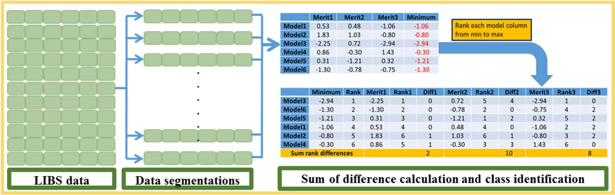
Figure 1.Calculation process of the LRC-SRD model in LIBS data.

Then the evaluation value ofai,2*xi,2…ai,n*xi,n=Xi aican be obtained based on the calculated vector ofai=[a i,1,ai,2,…ai,n]T,ai∈IRn×1.Subsequently, the distance between the real and evaluated is calculated asFinally,class identification is performed based on the minimum distancedi.

2.5.Other classification models

In addition to the LRC method,three additional classification methods,linear SVM,LDA and KNN were also implemented for comparison.SVM is a classifier with good classification performance that effectively identifies the category of each sample by constructing a hyperplane or a set of hyperplanes in a high-dimensional space [27].Currently, SVM has been applied in multivariate classification and regression problems.KNN is another commonly used classification model, the main idea of which is to calculate the similarity between a sample andksamples.If most of theksamples belong to a certain category,then the sample also belongs to this category[28].Notably, the similarity is usually presented by the Euclidean distance.LDA is a supervised learning dimensionality reduction technology that uses the projection method to achieve high classification performance in the case where the variance between the classes is the largest and the variance within the classes is the smallest [29].

2.6.Sum of ranking difference (SRD) and calculation process of the LRC-SRD model

The SRD,as a simple and effective algorithm,was originally proposed to solve the similarity problem among methods or models [30, 31].With the understanding of the SRD algorithm, many studies have explored the application range of SRD, which has been widely used to perform variable selection [32], identify model parameters [23] and select columns in chromatography [33].This study combined the LRC algorithm and SRD algorithm to further improve the performance of the LRC classifier.Thus, the SRD method is explained in relation to the present topic of LRC-SRD method.Based on the above statement of the LRC principle,four distance values were obtained when the LRC classifier was used to predict an unknown sample.

The 30 267 full variables of LIBS data were evenly and continuously divided intoNsegments.NLRC classifiers were obtained and applied to predict the unknown sample.As a result, one matrix with four rows (predictive distance value)andNcolumns (NLRC classifiers) was prepared to calculate the SRD value for each sample.When the input matrix was prepared, the standard sequence vector was first obtained based on the SRD algorithm.In this study, the standard sequence vector consisted of the smallest distance element in each row.Then, these selected elements of the standard sequence were sorted from small to large according to the value.Subsequently, each column was also rearranged from small to large, and the serial number of each element in each column was also changed accordingly.After the above calculation,the serial number of each column was compared with the serial number of the standard sequence column, and the absolute difference values between the above two columns were computed.Finally, the SRD value of each column was obtained by summing the differences between the reference column and each column.A relatively small SRD value corresponds to a stable and balanced model.Therefore, the prediction process of an unknown sample was carried out by finding the smallest SRD value.

To facilitate the understanding of the LRC-SRD calculation process, figure 1 was drawn to illustrate the whole implementation process using a specific example.According to the analysis of previous paragraph, LIBS data were first divided into several segments.Then LRC classifiers were established based on the divided segment variables.Notably,to easily understand the calculation process of the SRD algorithm, six classifiers (model 1–model 6) were used to calculate the distance(merit 1–merit 3).As shown in figure 1,a matrix with 6 rows and 3 columns was obtained and regarded as the SRD input matrix.Subsequently, a standard sequence consisting of the minimal value in each row was extracted from the matrix,and then the standard sequence was ranked in descending order.As the same time, all models were also ranked with the change of standard sequence and the sequence number of each merit (rank 1–rank 3) was also obtained.At last,the SRD value of each merit was calculated by computing the sum of absolute difference between rank and corresponding rank of merit.Consequently, the category with the smallest SRD value was identified as the prediction category.Above explanation is a simple illustration and more detailed information about the SRD algorithm example is provided in the references [30, 33].

Figure 2.Average spectral LIBS profiles of five groups of Tegillarca granosa samples.

2.7.Evaluation of model performance and algorithm implementation

To assess the performance of all classification models simply and accurately,in this study,a confused matrix containing the classification results of each sample and accuracy was used to evaluate the classification performances.For accurate analysis, a classification model should have high performance in term of accuracy, sensitivity and specificity.In this work, all algorithms were programmed by our research group and all calculations were run by using MATLAB 2015b (The Math Works, Natick, USA).

3.Results and discussions

3.1.LIBS spectral profiles of Tegillarca granosa

As shown in figure 2,five average LIBS spectra from four heavy metal-contaminated groups and the healthy group are presented and each spectrum contains a total of 30 267 variables in the spectral range of 217–800 nm.Generally,the spectral curve,with several hundred emission lines,is complex and similar in spectral profile among the five groups.First,several excitement lines with great intensity were identified on the basis of the National Institute of Standards and Technology(NIST)database such as K I(766 and 770 nm),Na I(588.9 and 589.5 nm),Ca I(422.7 nm),and Ca II (393.3 and 396.8 nm).In addition to these highintensity excitation lines,many low-intensity emission lines were also identified based on the NIST database such as C,Al,Si,and Cl.Unfortunately, the characteristic lines of the heavy metal pollution elements Pb, Zn and Cd could not be identified in the spectral profiles.The possible reasons are the matrix effect [34]and self-absorption [35], which lead to disturbance, absorption and disappearance of these excitement lines inTegillarcagranosa.Thus, it was difficult to distinguish different groups only by visual observation on the LIBS profile, and suitable machine learning methods should be performed to further utilize the LIBS data.

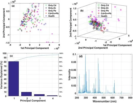
Figure 3.PCA analysis results of the 2D score plot(a),3D score plot(b),scree plot(c)and loading plot(d)for Tegillarca granosa LIBS data.

Table 1.Classification results of four classifiers KNN, LDA, SVM and LRC.

3.2.Exploratory analysis

Figure 4.Accuracy of the LRC classification model under different division ratios and different segments:(a)calculated results under 0.5–0.6 division ratios and 10–100 segments, (b) calculated results under 0.7–0.8 division ratios and 10–100 segments.

When high-dimensional data are analyzed,it is suggested first to perform a preliminary exploratory analysis,which will help with further data structure comprehension and facilitate subsequent analysis.Based on this idea, the most used dimensionality method of PCA was carried out to determine the sample and variable distribution.Figure 3 shows the PCA results as score, scree and loading plots using the PCA algorithm.As seen in figure 3(c),contribution rates of the PCs are reduced from more than 80% to less than 5%.The contribution rates of the first two and three PCs are approximately 90% and 95%, respectively.Based on the extracted PCs, the sample distributions of the five groups in 2D and 3D spaces were plotted.The distribution of these five groups of samples overlapped completely, and the healthy group and heavy metal pollution group could not be accurately separated.This may be caused by the similar LBS spectral profiles among the five groups.Therefore, it was difficult for PCA to distinguish different types ofTegillarca granosasamples only by observing the underlying structure of LIBS data.There are two possible reasons for this phenomenon.The first one is that the uncorrelated relationship between PCs just can provide limited information for understanding dataset structure.Another possible reason is that the structure of LIBS data is nonlinear,which means that the linear (classic) PCA cannot fully analyze the variables information to explore the data structure.In addition to the sample distribution,the loading plot was also generated based on PCA calculation result.Figure 3(d) shows the loading value of 30 267 full variables in the first PCs.It can be found that almost all variable’s loading value is large than zero and the profile is similar to the LIBS profile.That is, those variables having large intensity value have large contribution to the first PCs.By analyzing the calculation process of PCA,the possible reason behind this phenomenon is the positive correlation between the original LIBS spectral variables.This result demonstrates that LIBS spectrum is a kind of linear correlation data.Therefore,those variables with large loading value may play a more important role in the performance of the final model.Although some informative variables can be observed in the loading plot, the efficiency of these variables should be further validated in the following model.Comprehensive analysis of the above results indicated that a suitable classifier was needed to establish the classification model to further explore the possibility of rapid detection of the heavy metal pollution inTegillarca granosasamples.

3.3.Calculated results of the KNN, LDA, SVM and LRC classification models

To qualitatively detect the heavy metal pollution of theTegillarca granosasample and validate the power of the LRC classification model,150 samples were divided randomly into training and testing sets at a ratio of 3:2.As a result, 90 samples in the training set and 60 samples in the testing set were used to calibrate the classification model and validate the performance of the classifier, respectively.In addition to the LRC model, three additional commonly used classification algorithms, KNN, LDA and SVM, were also applied to create the classification models.Then, four confusion matrices of the testing set sample were obtained to present the classification result and the corresponding results were shown in table 1.For a confusion matrix plot, each column of the confusion matrix represents the true sample category, each row represents the predicted sample category, and the diagonal line in the confusion matrix indicates the number of correctly classified samples.In addition, the gray rows and columns in the confusion matrix indicate the proportion of samples correctly classified in the corresponding row or column.The overall accuracy is presented in the right corner of the confusion matrix.In table 1, it is clear that the LRC classification model has the best performance,and the overall accuracy reached 0.75.When the KNN, LDA and SVM models were considered, they had accuracies of 0.30, 0.40 and 0.42, respectively.The results mean that these models were not suitable methods to establish the heavy metal pollution detection model forTegillarca granosasamples, for which there are three possible reasons.The first reason is that there are too many input variables in the model, which may introduce noise and useless variables into the calculation model and lead to poor performance in terms of accuracy.On the other hand,the KNN,LDA and SVM algorithms can only handle relatively low-dimensional (tens to thousands of dimensions)data compared with the LRC algorithm,which is more suitable to process high-dimensional data.In this study,there were 30 267 variables in the LIBS data, which make LRC more suitable for analysis than the other models.In addition,LRC is a no-parameter model that does not have the process of model training.Consequently, it can avoid model instability caused by unsuitable parameters and give accurate test results.Compared with the performance of the other three classification models, the LRC classifier had significantly higher accuracy, but there was still room for improvement.

3.4.Analysis of the results from the LRC-SRD model

Based on the above analysis, the accuracy of the LRC classification model was still insufficient, although the LRC model had an overwhelming performance in terms of accuracy compared to the other classifiers.To further improve the performance of the LRC model, the SRD algorithm was considered and combined with the LRC method to establish a more efficient LRC-SRD classification model.Prior to selecting the optimal model, two parameters of the sample division rate and the number of variable segments had to be optimized.In this study, the ranges of the sample division ratio and segment number were set as 0.5–0.8 with a step of 0.1 and 10–100 with a step of 10, respectively.Then, all combinations of the sample division ratio and variable segment number were considered to establish the LRC-SRD models,and the calculated accuracy is shown in figure 4.The accuracy was different when different proportions of samples in the dataset were divided into the test set.When all variables were input into the LRC model, four different results were acquired,and the accuracy was in the range of 0.64–0.75.The best model was that with a sample division ratio of 0.6, the accuracy of which 0.75.In contrast,the least sufficient model was that with a sample division ratio of 0.5, exhibiting an accuracy of 0.64.When the sample division ratios were 0.7 and 0.8, the accuracies were 0.71 and 0.73, respectively,which were higher than that of the model with a sample division ratio of 0.5.On the other hand, a different but improved accuracy was obtained from the LRC-SRD model when 30267 variables were divided into 10–100 segments to create the LRC-SRD classification model.It can be found that all LRC-SRD classification model performance were remarkably improved.The highest accuracy was 0.93 from the combination ratio of 0.6 and 40 segments, and the increased ratio reached 24.4% and increased the accuracy from 0.75 to 0.93.All the above results proved the effectiveness of the SRD algorithm in improving the performance of the LRC classification model.

All models were carried out under different combinations of division ratios and variable segments.Four confusion matrices from the four best combinations under a sample division ratio of 0.5–0.8 were plotted and are shown, and more detailed sample classification information can be observed in table 2.It can be concluded that all samples in categories 5(healthy group)and 3(Pb pollution group)could be correctly classified,and 100%accuracy was obtained.The Zn and Cd pollution group samples can basically be classified correctly(accuracy from 77.8%to 100%).Category 4(heavy metal mixed pollution group) had the poorest classification result except for the result in that of the 0.6 ratio model, and only half of the samples were classified correctly (accuracy from 55.6% to 66.7%).This phenomenon may be caused by the fact that healthy samples have greater differences with the individual heavy metal polluted groups than that with the mixed polluted group.Conversely, the similarity among the mixed heavy metal polluted group with the other three heavy metal pollution groups may be the reason why the mixed heavy metal pollution samples could be accurately separated from other groups.However, it could be concluded that it is feasible to distinguish healthyTegillarca granosasamples from heavy metal polluted samples.In addition, the performance of the LRC classifier was significantly improved whenthe SRD algorithm was used to detect heavy metals in theTegillarca granosasamples.Although this study demonstrated the effectiveness of the method,this phenomenon may be due to two reasons.The first reason is that LRC is a method with good performance when processing highdimensional data.This is also the reason why LRC has a higher accuracy than that of the classifiers.That is,a generally satisfactory accuracy laid a solid foundation for the subsequent calculation,which makes the SRD algorithm suitable for combination with the LRC model.Another possible reason is that the variable information of LIBS data was used more rationally.Many classifiers can be established based on the variable segments when 30 267 variables are divided into several segments,and the calculated distance from each classifier is put into the SRD algorithm.During the computation of SRD, the calculation mechanism can be compared to a process of voting by many classifiers.Therefore,those classifiers based on useless variables and noise could be ignored in this process.This calculation process is equivalent to a consensus calculation that can make full use of spectral information.As a result, optimal performance was obtained by the LRC-SRD model.Overall,SRD coupled with the LRC algorithm is an efficient and powerful combination to comprehend high-dimensional LIBS data.The calculated results in table 2 validated this conclusion.

Table 2.The classification results of the LRC classifiers under combination of division ratio and segments: the combination of division ratio 0.5 and variable segment number 30 segments; the combination of division ratio 0.6 and variable segment number 40;the combination of division ratio 0.7 and variable segment number 30, and the combination of division ratio 0.8 and variable segment number 10.

4.Conclusion

This study investigated the feasibility of the LIBS technique for determining heavy metal contamination inTegillarca granosa.First, four classic classification algorithms were applied to establish the detection model for heavy metal pollutedTegillarca granosasamples.Only the LRC method achieved a relatively applicable accuracy (0.75), and the performances of the other model were very low that the models cannot be used in practice.To further improve the detection accuracy, a novel and effective framework called LRC-SRD was proposed to establish a more accurate detection model forTegillarca granosasamples.Compared with the single LRC model, a significant improvement was obtained by the LRC-SRD classification model, and the accuracy increased from 0.75 to 0.93.Moreover, all model performances were improved when SRD was combined with the LRC algorithm.Thus, the proposed LRC-SRD algorithm is an effective method to establish the classification model for dealing with high-dimensional LIBS data.In conclusion, the LIBS technique coupled with the LRC-SRD framework was an alternative method to rapidly detect heavy metal pollution inTegillarca granosasamples.

Acknowledgments

This work was supported by the Natural Science Foundation of Zhejiang Province (No.LY21C200001); National Natural Science Foundation of China (No.31571920); Wenzhou Science and Technology Project (No.N20160004) and Wenzhou Basic Public Welfare Project (No.N20190017).