Dujia Yang,Xiaowei Qin,*,Xiaodong Xu,Chensheng Li,Guo Wei

1 University of Science and Technology of China,Hefei 230026,China

2 CAS Key Laboratory of Wireless-Optical Communications,Hefei 230027,China

Abstract:Reinforcement learning can be modeled as markov decision process mathematically.In consequence,the interaction samples as well as the connection relation between them are two main types of information for learning.However,most of recent works on deep reinforcement learning treat samples independently either in their own episode or between episodes.In this paper,in order to utilize more sample information,we propose another learning system based on directed associative graph(DAG).The DAG is built on all trajectories in real time,which includes the whole connection relation of all samples among all episodes.Through planning with directed edges on DAG,we offer another perspective to estimate stateaction pair,especially for the unknowns to deep neural network(DNN)as well as episodic memory(EM).Mixed loss function is generated by the three learning systems(DNN,EM and DAG)to improve the efficiency of the parameter update in the proposed algorithm.We show that our algorithm is significantly better than the state-of-the-art algorithm in performance and sample efficiency on testing environments.Furthermore,the convergence of our algorithm is proved in the appendix and its long-term performance as well as the effects of DAG are verified.

Keywords:directed associative graph;sample efficiency;deep reinforcement learning

I.INTRODUCTION

Developing from animal learning and parameter perturbation adaptive control,reinforcement learning(RL)is a type of machine learning algorithms which is most closely related to human decision-making[1].Besides,with the powerful neural networks,parametric deep learning methods keep making breakthrough in image understanding[2],natural language processing[3],etc.Marrying deep neural networks(DNN)with RL,deep reinforcement learning(DRL)is the most notable RL in academia and journalism for its successful applications in video games[4],robot control[5],autonomous driving[6],etc.DNN brought DRL great representational power for complex environment except for a lot of problems:spatial complexity,computational complexity and sample complexity[7].To solve these complexity problems,a lot of time,manpower and material resources are consumed,especially for model-free DRL,which is more practical and focused recently.What is worse,the sample costs for real-world applications,e.g.,mobile communication and adaptive bitrate algorithms in MPEG-DASH,are far higher when compared to video games,which hinders its wide application in society.

In this paper,we focus on how to solve the sample complexity problem by improving the sample efficiency for the value-based model-free DRL.According to[8],one of the primary intrinsic sources of sample inefficiency is the incremental parameter adjustment in DRL.To avoid the possible ‘catastrophic interference’in early learning,the adjustments of neural networks must be quite small[9].There are many recent works focusing on improving sample efficiency,including many variants of Deep Q-Network(DQN)[10]and episodic DRL.DQN and its variants store samples in replay memory(RM)and sample batches randomly and independently to update the algorithms.As for episodic RL,it leverages episodic control[11],which builds episodic memory(EM)by recording highly rewarding experiences in each episode independently.MFEC[12],NEC[13],EMDQN[14],EVA[15],HE-EMDQN[16]are typical episodic RL algorithms.

It is known that RL is considered as a sequential decision making problem which can be modeled as markov decision process mathematically[17].In consequence,the interaction samples themselves as well as the relationship between them are two major information for learning.It is worth noting that the complete connection information is also useful in not only computing the value of existing states but also estimating the value of unknown states.However,DQN and its variants ignore the relationships between samples in one episode and treat them as independent ones during the batch sampling.As for the episodic RL algorithms mentioned above,they combine samples from the beginning to the end of one episode into episodic data and use them as a whole in the training progress.Nonetheless,different episodic data is treated independently as well.In other word,they do not take a better use of the whole associative relationships of all samples among all episodes.

Inspired by cooperation and competition between the massively parallelized neural architecture in brains[18],we propose a sample-efficient method for DRL which is composed of three information utilization modules:deep neural network,episodic memory and directed associative graph(DAG).DNN and EM are two learning systems that learn from samples independently or connection relation within episodes partially.As for DAG,it’s a graph which is built on the whole connection relation among trajectories generated by the agent in real time.Through planning with directed edges on DAG,we introduce another learning system to estimate state-action values.In brief,the main contribution of this paper is described as follows:

(1)Planning on DAG:We build a directed associative graph among all samples and their associative relationships in real time.Taking advantage of DAG,values can be propagated along the current state through this associative graph.So we propose a method of planning on this real-time DAG to find all possible next N-step states and leverage Bellman equation[19]and values from EM or target network to offer a proper estimation for current state,even it is an unknown state for EM or DNN.We show the convergence of this planning in Appendix VI.Experiments also shows that this estimation is important for unknown states,especially in the early stage of training.

(2)Making better use of the sample information:We introduce three learning system to utilize the sample information(samples as well as their association relationships)from different perspectives.Firstly,the whole sample information is updated in DAG in real time and the planning on DAG is executed to estimate the target value from the near-global perspective.Secondly,when one episode ends,the episodic data is calculated wholly to update EM.Finally,samples are sampled randomly and independently to constitute batches at the stage of update.When combing these supervised values generated by DNN(target network),EM and DAG into the loss function,sample information,especially associative relationships,is much better utilized.Experiments shows that parameters updating in DRL are far more sample efficient in this way.

The remainder of this paper will be organized as follows.Firstly,the background of RL is introduced in Section II.Then we will give a brief review of related works recently in Section III.In Section IV,we will introduce the basic framework and the key works of our algorithm in-depth.Experiment process and result analysis are provided in Section V to demonstrate the effectiveness of our model.Section VI concludes the paper with some discussions as well as future works.

II.BACKGROUND

2.1 Reinforcement Learning

Reinforcement learning is usually modeled as markov decision process(MDP):whereandare state space and action space respectively,is reward function,is the transition probability between states ands0is the initial state.At the time stept,the agent observes a statest∈and takes an actionaccording to the policyπ(a|st).Then the environment transfers to a new statest+1with probabilityP(st,at)and returns a scalar rewardrt∈Rto the agent.The final goal of the agent above is to learn an optimal policyπ∗that is able to get the maximum expectation of cumulative discounted returnwhereγ∈[0,1]is the discount rate.

Another important concept is value function.The state-action value functionQπ(s,a)provides an estimation of the expected amount of discounted return over the future,when starting from states,actionaand following a policyπ.The function can be computed recursively with dynamic programming:

For value-based RL,the agent tries to learn an approximation optimal policy by acting greedily on these values.To achieve this goal,one way is to follow the optimal value function who satisfies the Bellman equation[19]:

One of the most classic early RL algorithms is Qlearning[20].It is a table-based simple method and uses the well-known temporal difference(TD)errors to iteratively updateQ(s,a)as well as find the optimal value:

2.2 Deep Q-Network

Combining deep learning with Q-learning,DQN is able to solve the problem of both capacity limitation and sample correlation of the traditional table-based RL.It is a classic parametric DRL model which is parameterized by weights and biases denoted asθ.Instead of Q table,state-action values are estimated by DNN denoted asQ(s,a|θ).At the stage of update,a mini-batch of experience is sampled randomly from the RM.Like Q-learning,TD errors are also calculated as the loss function:

whereθEis the parameters of evaluation network and target valueyt=rt+γmaxa′Q(st+1,a′|θT)is computed by the target network with parametersθT.θEis updated by minimizing the loss function through gradient descent andθTis copied toθEin every setting steps.

2.3 Episodic Memory

The term ”episodic memory”is a biological concept,which is coined by Endel Tulving[21].It is an explicit memory who stores the retrieval of contextual information pertaining with a specific event or experience that has occurred.In RL,the episodic memory is stored as the encountered state and the reward that followed for the episodic environment.Different from the traditional RL algorithms such as table-based Qlearning or parameter-based DQN,this method is built on the process of recollection among a long sequence of samples in one episode(more commonly the whole episode)which is regarded as an event or instance.

The environment we considered in this paper is episodic,so it is suitable for episodic memory.Each episode ends in a special state called the terminal state which is followed by a reset to a standard starting state or to a sample from a standard distribution of starting states[17].For episodic RL,each episode will end with finite steps denoted asT.Then,the accumulated discounted return at thetth time step is calculated aswhere the discounted factorγ∈[0,1]is mainly used to balance the importance of current and future rewards.As for the episodic reward,it is the sum of total real rewards without discount in each episode:Generally,it’s an indicator with practical significance,e.g.,total score of players in each episode of video games.In practice,RL takes advantage of the accumulated discounted return to train its algorithm,while uses the episodic reward(Score in this paper)to show its performance intuitively.

Based on episodic control,EM is a tabular module which stores an explicit record of the past experience.There are many EM module in previous works and we adopt the one in HE-EMDQN,which is a hash table defined asQEM(s,a).When one episode is finished,the whole episode data is collected to calculate allRt(st,at),denoted asand the EM is updated byepisodically.

III.RELATED WORK

In this section,we will review the related works of various recent RL algorithms and analyze the way they utilize sample information.

3.1 Deep Reinforcement Learning

DQN is the first algorithm that combines deep learning with Q-learning and surpass human-level performance on many Atari 2600 games.Double DQN[22]addresses the overestimation bias by decoupling action selection and value estimation in target network.Prioritized Experience Replay[23]further improves Double DQN by preferentially replaying samples in replay buffer according to TD errors.Authors in[24]propose a dueling DQN that splits value function into state value and advantage value.Distributional Q-learning[25]learns a categorical distribution of discounted returns,instead of estimating the mean.However,samples in these DRL algorithms are considered to be independent and no relation is used directly.Instead of just one step learning in DQN,multi-step bootstrap targets[26]show faster performance in propagating newly observed rewards.Optimality tightening method[27]tightens the optimization of DQN via constraints which is calculated by exploiting multi-step states before and after the current state in experience replay.Retrace(λ)[28]incorporates on-policy short sequences from the memory instead of single transition into off-policy learning targets.Nonetheless,only multi-step related samples in one episode are utilized in these algorithms.

3.2 Episodic Reinforcement Learning

Episodic RL keeps an explicit record of past episodic events and use this record directly as a point of reference when the agent is going to make new decisions.Model Free Episodic Control(MFEC)is one of the first few works on episodic RL[12].This model is non-parametric and data-efficient when compared to traditional gradient-based DRL.Neural Episodic Control(NEC)[13]introduce a key structure called differentiable neural dictionary(DND).DND is an episodic memory module and allows estimating state-action values according to the similarities between stored neighbor states.Ephemeral Value Adjustments(EVA)[15]modifies the value for action selection predicted by neural network with an estimated value function by planning over nearest experience tuples from the replay buffer.EBU[29]performs backward updating by sampling episodic sequence instead of the random mini-batches in experience replay.As for AE-DDPG in[30],the authors design a new experience replay policy which mixes RM with“HMemory”who memorizes the whole episodic sequence that gets the highest score at present.EMDQN[14]combines parametric DQN module with non-parametric episodic control module for the purpose of improving both sample efficiency as well as module generalization.Recently,authors in[16]proposes a new sample-efficient reinforcement learning architecture called HE-EMDQN which introduces a new EM module and incorporates some episodic thoughts above into the key components of DRL.HE-EMDQN shows better sample efficiency than EMDQN.The episodic information of sample relation is contained through different EM modules in those episodic RL algorithms.However,algorithms mentioned above only take advantage of relation in their own episodes.The whole connection relation of all samples among all episodes is ignored.

Based on EMDQN,ERLAM[31]builds a periodically updated graph on top of states in memory to form a so-called associative memory which is only used to fasten the update of episodic memory.SoRB[32]builds a directed graph on top of states in replay buffer and combines planning via graph search and goal-conditioned RL.Notwithstanding,this planning is to find the sequence of waypoints not to estimate the real value of states which is more general for RL.QG-DDPG[33]applies a subgraph which is simplified by a zero action hypothesis with relation information discarding to continuous motion environments.This graph pruning is suitable for deterministic environments,but ignores the randomness of the truncated states in near-deterministic or stochastic environments.DGN[34]proposes graph convolutional RL in multi-agent scenarios,where the graph is built on the multi-agent environment and the relation is the interplay between agents.However,this graph is used to improve the information usage among agents rather than among samples.

3.3 Applications of Deep Reinforcement Learning in Communications

Recently,RL,especially the powerful DRL,has been introduced to solve various problems effectively in obtaining the optimal policy in communications.Authors in[35]use DQN to address the dynamic channel access and interference management among small base stations who share unlicensed channels in 4G LTE network.DRL-DCA[36]models the satellite system as the agent and the channel as the action,then the system’s optimization problem is solved by DQN effectively.In addition to the applications in network access,D-DASH[37]combines DQN and MPEGDASH to solve the problem of Adaptive Bitrate(ABR)control in dynamic networks,and can provide much better Quality of Experience(QoE)when compared to the traditional algorithms.Chenet al.[38]propose a deep reinforcement learning based algorithm to optimize the resource allocation problem in intelligent transportation system,which achieves faster convergence speed and higher performance in reducing perception-reaction time during the simulation.Based on DQN,Xuet al.[39]design a joint resource allocation scheme for solving the complex optimization problem and improve the communication and computing efficiency greatly.As for network security,authors in[40]propose a DQN-based power control scheme for IoT devices to improve the transmission efficiency and save energy without the special knowledge of IoT topology and the jamming model.

Although DRL does a good job in addressing many problems in communications,large number of samples are needed for training because of its sample inefficiency.Most of the existing works rely on simulated datasets,because samples in real world are not easily accessible.Taking ABR control problem in video service for example,video samples,especially those with user experience score from crowdsourcing,are very hard and expensive to collect.Fortunately,developed by software,video games are virtual environments and their security,difficulty,task type and duration can be controlled artificially.What’s more,video games can provide almost unlimited samples for DRL within a short time.In consequence,video games have become a perfect,unique environments and the most popular field in artificial intelligence[41].

In this paper,our work focuses on how to improve the sample efficiency of DRL,so we use the benchmark environments of video games to verify the effectiveness of our algorithm.Even so,we think this work is suitable to solve the problem of sample efficiency that perplex many work in communications as well.

IV.ALGORITHM WITH DIRECTED ASSOCIATIVE GRAPH

The key point of our work is taking advantage of the sample information,i.e.,interaction samples as well as the connection relation between them.To achieve this goal,we take DQN algorithm as the basic DRL and introduce a comprehensive utilization architecture on it,which is illustrated in Figure 1.The solid lines in Figure 1 represent the workflow of value transfer,while the dashed lines are the propagation path of single sample or sample sequence.At the time stept,the agent observers statestfrom the environment and takes actionataccording to the exploration strategy of DRL.Then the environment feeds back new statest+1and rewardrtto the agent.The sample which contains all experience informationet=(st,at,rt,st+1)is stored in RM.Meanwhile,the DAG receives the element which contains connection relationgt=(st,(st,at,st+1))and update itself in real time.When this episode comes to an end,EM is updated in episodic control manner through the whole episodic dataT={e1,...eT}(also called trajectory).At the stage of every updating,a mini-batch are sampled from RM and are pushed to three learning system to get three target values.The loss function calculates each loss respectively and combines them to update the DQN networks further.Details are shown in Algorithm 1 and we will introduce the algorithm in the next sections.

4.1 Directed Associative Graph

Algorithm 1.Directed associative graph for DRL.1:Input Nstep,freq update1,freq update2 2:Initialize T,RM,EM,G 3:for each episode do 4:for t=1,2,3,...T do 5:Receive state st from environment 6:Select action at by ∊-greedy or other policy 7:Take action at,observe next state st+1 and receive reward rt 8:Append(st,at,rt,st+1)to RM and T 9:Update DAG G with gt=(st,(st,at,st+1))according to Eq.(5)10:if t mod freq update1==0 then 11:Sample mini-batch and for all samples:qθT=rt+γ maxa′Q(st+1,a′|θT),search in EM to get qEM,planning on G to get qDAG.12:Calculate mini-batch’s loss via Eq.(12)and update θE 13:end if 14:end for 15:Update EM with the whole episodic data T 16:Empty T 17:if t mod freq update2==0 then 18:Copy θE to θT 19:end if 20:end for

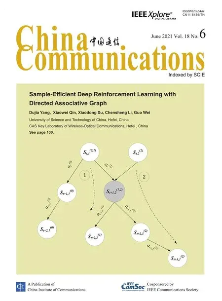
We build a directed associative graph on top of all trajectories generated by the agent in the environment to store trajectory information.As shown in Figure 2,each node in DAG corresponds to a state and is bridged by the directed edges who represent the relation between them according to the transitions in each trajectory.The dash lines in Figure 2 represent some trajectories,while the bracketed superscripts of elements represent the trajectory to which the elements belong.In our paper,the observation of high dimensionotfrom the environment is mapped to an embedding statestthrough an embedding function.There are many embedding functions,such as gaussian function[42],convolution neural network[13],simihash[43].For the sake of simplicity,we use the gaussian projection which approximately preserves relative distance in the original space according to the Johnson-Lindenstrauss lemma[42].The directed associative graph is defined as

Figure 1.Comprehensive utilization framework of samples.

Figure 2.Directed associative graph.The solid lines are the real edges in the graph,while the dash lines represent some trajectories.Note that bracketed superscripts of elements represent the trajectory to which the elements belong.

andBis all states encountered by the agent at present.Specially,given a sampleet=(st,at,rt,st+1),we first regroup it as a graph elementgt=(st,(st,at,st+1)).Then the nodestis added to the graph if not exists,and we update the directed edge on the basis of(st,at,st+1)which meansstdirectsst+1under the actionat.Note that our DAG is updated in real time rather than periodically or episodically.

We use a structure of hash table to store the DAG,whose keys represent nodes and values store the directed edges.For the environment with state spaceSand action spaceA,the spatial complexity of building a complete DAG is|S|×|A|.In this paper,we embed the original state space of the environment into a lowdimensional space,i.e.,4,so this spatial complexity is not very big.Practically,we just use a hash table with a buffer of 2×106size,where the oldest elements will be removed when the buffer is full.

4.2 Planning on DAG

Planning is a concept in model-based RL that an agent samples experience from a model of the world to improve its policy without further interaction with the environment[44].Our DAG can be seen as a graphbased model of the world but not a complicated transition probability model.Planning on DAG is a way of recalling associated experiences and using these past experiences and their context relationships to improve model-free value estimates.Specifically,once the DAG is built,given state-action pair(st,at),we can find all possible next states or next N-step states(if exists).Through this planning,values can be propagated across steps to produce value estimateby Bellman equation[19].Taking one-step planning for example,is calculate as:

whereQM(st+1,a)is the target value estimated by EM or the target network in DNN:

Because of the randomness of environment and information compression of state embedding,a new state is unknown to DNN or EM,but its following state may exist in previous episode.For instance,a statest,1in current trajectoryT1in Figure 2 is unknown to DNN and EM.But through planning on this real-time DAG,we find that its next statest+1,2(the grey node)underathas already been experienced in previous trajectoryT2which is finished and updated with episodic values to EM.Thus,through Eq.(6)and Eq.(7),our algorithm is able to leverage both the fast reward prorogation of EM and the generation of DNN to estimate the value of this new state-action pair.

Figure 3.Testing curves of HE-EMDQN,EMDQN,DQN and DAG-HEEMDQN on representative games.Scores are smoothed using moving average over 4 testing epochs.Each game is run 3 times with different random seeds.

Practically,in order to shift the bias-variance tradeoff,Eq.(6)can be rewritten as N-step value estimatewhich is calculated through Nstep planning on DAG in the manner of recursion:

and the final value is calculated asQM(st+N,a)by Eq.(7).Sinceis calculated by Bellman equation,it will converge to unique optimal value through iterations.We show proofs In Appendix VI.

Thanks to the structure of hash table,the complexity of query on DAG is onlyO(1).As for the planning,its complexity isO(|A|N)in the worst case.Fortunately,since the final valuesQM(st+N,a)are mostly from EM which already contains long-term episodic information,the steps of planning on DAG can be set as a small value(N=2 in this paper).

It should be noted that different from the trajectorycentric planning in EVA,ouris planning on all state connection space not just within one trajectory.Besidesis calculated as a target value from another perspective for learning rather than for exploration.

4.3 Mixed Loss Function

As mentioned in the introduction,human beings are good at using a variety of learning,memory and decision-making systems to perform tasks effectively in different situations[18,45,46].Our work is inspired by this rapid complementary approach of decision making in the brain.Thus,we propose a sampleefficient method for DRL which is composed of three information utilization modules:DNN,EM and DAG.DNN and EM are two learning systems that learn from samples independently or connection relation within episodes partially,which is applied in EMDQN and HE-EMDQN.In this paper,we propose another learning system based on DAG which is built on the whole connection relation in trajectories.Values of stateaction pair(st,at)computed by target DNN(qθT),EM(qEM)and DAG(qDAG)are working as three target values for DRL:

We use the powerful DNN as the main structure and introduce two other learning systems,i.e.,EM and DAG to overcome the former’s shortcomings such as overestimation and sample inefficiency.In other word,these extra learning systems are used to optimize theDNN system.So we calculate these two loss separately and mix them into the loss function of DNN,in whichLEMandLDAGare added toLDNNas regularizer:

whereλEM,λDAG∈[0,1]are regularization hyperparameters.Obviously,whenλDAG=0,ourLis identical to the mixed loss function in[14,16].Furthermore,theLreverts to the standard loss function in DQN whenλEMandλDAGare both set to zero.

More supervised values from different perspectives bring DRL more information to learning.Under these circumstances,the parameter updating in DRL will be more accurate and as a result,the sample efficiency will be improved.

V.EXPERIMENTS AND ANALYSIS

Based on DQN,the recent work HE-EMDQN improves the sample efficiency of DRL by making use of episodic memory high efficiently.Therefore,we apply the framework of this paper to HE-EMDQN,which is called Directed Associative Graph for HEEMDQN(DAG-HEEMDQN).Apart from adding an extra structure of DAG,we only change the loss function to our mixed loss function while other parts unchanged.To verify the effectiveness of DAGHEEMDQN in sample efficiency,we test our algorithm on the benchmark suite of Atari 2600 games from the Arcade Learning Environment which is provided by OpenAI Gym[47].Environment in these games is high-dimensional,continuous and random with sparse rewards in some games.In a word,they are widely used for performance comparison in RL at present.Without loss of generality,we select 20 games of Atari 2600 according to the alphabetical order randomly to evaluate the performance of HE-EMDQN,EMDQN,DQN and DAG-HEEMDQN.The selected games are listed in Table 1.

Table 1.Score comparison of DQN,EMDQN,HE-EMDQN and DAG-HEEMDQN.

Table 2.Performance comparison on mean and median human-normalized scores over 20 games.

5.1 EXPERIMENTAL SETUP

The structure of DNN and the basic hyper-parameter settings of HE-EMDQN,EMDQN,DQN and DAGHEEMDQN are all set the same as[14].For EMDQN,HE-EMDQN and DAG-HEEMDQN,we choose the gaussian projection as the embedding function to embed the observation into a 4-dimensional state,which is used as the state key for the updating or query of EM too.What’s more,these 4-dimensional embedded states are also used as the nodes in our DAG.In addition,parameters in the comprehensive utilization framework of episodic memory(episodic module,mixed experience replay and episode adjusted exploration)in HE-EMDQN and DAG-HEEMDQN are set the same as[16].Specially,for DAG-HEEMDQN,the following hyper-parameters are tuned on Qbert,Enduro and Pong.We use hash table with buffer size of 2 million to store the DAG,from which the oldest sample is discarded to store the new one if it is full.The regularization hyper-parametersλEMandλDAGare set to 0.1 and 0.05 respectively.We set the N-step planning on DAG with a small step,i.e.,2.For the testing environment,the rewards in all games are clipped to[−1,1].

Finally,we train these four algorithms with 10 million frames and evaluate them every 250000 frames.During evaluation,every agent runs for 30 episodes with 30 no-op operations at the start of each episode[12].The final result of each evaluation is the average of these 30 scores.Each game is run 3 times with different random seeds.

5.2 Results

5.2.1 Results on games

Just as[10],we show the highest average testing score during every game’s training for score comparison among HE-EMDQN,EMDQN,DQN and DAGHEEMDQN in Table 1.This score is a common measure to show the best performance of an algorithm.From Table 1,we can find that DAG-HEEMDQN is far better than EMDQN and DQN on almost all games.For HE-EMDQN,our algorithm scores much higher on 17 games(85% percent on 20 games),while just slightly worse than the former on the other 2 games(scores are equal in Jamesbond).To see the comprehensive performance of all algorithms,we also compute human-normalized scores across games among these four algorithms in accordance with[22]:

Note that the ’random’ and ’human’ scores of all games are the same as shown by[10]which are common values.The mean and median human-normalized scores are summarized in Table 2.Apparently,DAGHEEMDQN performs considerably better than the other 3 algorithms in this comprehensive metric as well.

For further comparison,we also show the testing curves of 8 games during training in Figure 3.These curves outline the progress of average testing performance of all algorithms during the training with more details.Obviously,our algorithm performs quite better than HE-EMDQN both at the early stage and the final stage,especially in Breakout,FishingDerby,Hero and Krull.Taking Hero for example,the final results of DAG-HEEMDQN in Table 1 is the best one,which is almost twice as much as HE-EMDQN.For the testing curves,it takes HE-EMDQN more than 9 million training frames to get the steady best average testing score where only 5 million training frames are needed for DAG-HEEMDQN.

In brief,DAG-HEEMDQN shows best performance in both testing scores and testing curves.Through the comparison with HE-EMDQN,our improvement measures of DAG and mixed loss function do help improve the performance as well as sample efficiency for DRL.

5.2.2 Long-term performance

In order to see the long-term learning ability of our algorithm,we also train these four algorithms with 20 million frames on 4 games.The selected games and the real training curves are shown in Figure 4.It is worth noting that the real-time training mean scores are the moving average scores of last 100 episodes during training.A better training curve means that the algorithm has better learning capabilities,and thus are more likely to get better testing performance.

The results show that with the increase of training samples,our algorithm still maintains better training performance in Hero,Krull and Zaxxon.As for Qbert,although the final performance is similar,our algorithm converges to the optimal performance much earlier than HE-EMDQN,i.e.,more sample efficient.Therefore,we believe that our algorithm will get better performance or better sample efficiency at least when more samples are available.

5.2.3 Effects in Evaluating Unknown State-action Pairs and Mixed Loss Function

To understand how our algorithm works with improved performance,we do extra analysis on its effects in evaluating unknown state-action pairs and mixed loss function with experiments in Figure 5.

Figure 4.Training curves with 20 million training frames on 4 games.The scores are smoothed using moving average over the last 100 episodes with the same random seed.

Figure 5.Left column:The rate of estimate unknown stateactions at different training stages.Right column:The bach mean scores of three target values qθT ,qEM and qDAG .

As mentioned above,the way that planning on realtime DAG to find all possible next N-step states and leverage Bellman equation with values from target network as well as EM makes our algorithm own the ability to estimate the unknown state-action pairs.Firstly,we plot the rate of unknown state-action pairs in minibatch during updating,which are not in EM but can be estimated by planning on DAG.Results are shown in the left column of Figure 5.We see that this estimation is mainly effective in the initial stage of updating,and gradually weakens as the training progresses.This fits the common intuition that the agent is more inexperienced to the environment at the beginning,where not enough information from EM or DNN is available.It can only obtain a value estimation through planning on DAG until EM is filled with more and more information as the training continues.From the curves in Figure 3 and Figure 4,we can also find that our algorithm performs not bad or even much better at the beginning in many games.Therefore,we believe that making up for the lack of EM estimation for unknown state-action pairs is an important reason in improving sample efficiency,especially in the early stage(less than 4 million frames).

DQN tends to overestimate values for its maximization operation over both action selection and target value calculation[22].Double DQN reduces the overestimation by estimating the target value independently from the action selection.Similar to this idea,we introduce another two learning system for the estimation of target value independently in this paper.The right column of Figure 5 are the batch mean scores of three target values during the updating of DAGHEEMDQN.Note that each point on the curve represents the mean value of every 1000 updates.We can see thatqθT,qEMandqDAGshow different value estimation at different update stages.Oriented from nonparametric EM whose rewards are fast propagated,qEMcan help alleviate overestimation ofqθTin the initial stage.Besides,the parametric DNN is good at function generalization and long-term learning.As for DAG,it explores the connection relationship between samples and realizes the estimation of the target value from the near-global perspective further.Thus,we argue that combining the three different target values to form the mixed loss function will do help in improving algorithm performance continuously.

VI.CONCLUSION

In this paper,we build a directed associative graph on the whole connection relation among trajectories in real time.On this basis,we propose a new method which leverages the integrated information utilization modules,i.e.,DNN,EM and DAG to make better use of the sample information.They are three learning systems and offer DRL algorithm with different perspectives.Then a mixed loss function generated by this three learning systems is used to improve the efficiency of the parameter update in DRL.We show across the Atari games that our algorithm is significantly more powerful and sample-efficient than the basic episodic DRL algorithm HE-EMDQN.Furthermore,we also demonstrate the convergence of our algorithm and analyze the long-term performance as well as the effects of DAG with extra experiments.In conclusion,through making high efficient use of sample information,our algorithm makes difference in improving sample efficiency for DRL.In the future,we will extend our works on:1)finding better embedding function to build the directed associative graph;2)combining other algorithms like ERLAM to expand the usefulness of DAG;3)adjusting our work to policy-based RL to solve the problem of sample efficiency in real world,such as mobile communication and adaptive bitrate algorithms in MPEG-DASH;4)applying other biologically inspired ideas to DRL to improve the sample efficiency further.

ACKNOWLEDGEMENT

This work is supported by the National Key Research and Development Program of China,2018YFA0701603 and Natural Science Foundation of Anhui Province,2008085MF213.

APPENDIX

Let value function estimated through planning on directed associative graph bewhere the state space,action spaceand reward spaceare all finite space.Denote the Bellman operator asB,the value function asand a map.Then,converges to the unique optimal valuethrough repeated iteration.

Proof.Givenstate-actionpair(s,a),letPDAG(s′|s,a)be the transition probability between states.Letrepresents the starting element and define an iterative sequenceby

whereγ∈[0,1)is the discount rate andn∈N.Besides,for any two elementsandin,the distance metric is defended as

Then,for any state-action pair(s,a),the derivation process is described in Eq.(16).

In consequence,the Bellman operator is a contraction mapping whenγ∈[0,1).According to Banach fixed point theorem[48],for the fixed optimal pointQDAG∗,we can get

Therefore,value function estimated through planning on directed associative graph will converge to the unique optimal value through repeated iteration.