Yucheng Yang(杨雨成), Teng Wu(吴腾),†, Jianwei Zhang(张建玮), and Hong Guo(郭弘),‡

1State Key Laboratory of Advanced Optical Communication Systems and Networks,Department of Electronics,and Center for Quantum Information Technology,Peking University,Beijing 100871,China

2School of Physics,Peking University,Beijing 100871,China

Keywords: atomic comagnetometer,atomic magnetometer,domain wall,axions and axionlike particles

1. Introduction

It has been indicated by many astrophysical and cosmological observations that only ～5% of the universe is made up of standard model (SM) matter, and the rest is dominated by dark energy (73%) and cold dark matter (23%).[1]However,we have not yet been able to explore the characteristics of dark matter in the laboratory. Dark matter is known to be nonluminous and non-baryonic,and its interactions with SM particles are very weak.[2]Weakly interacting massive particles(WIMPs) were thought to be the components of dark matter.Nonetheless,WIMPs have not yet been found within the background limit set by neutrino interactions, and it is necesary to consider other dark matter candidates.[3]Ultralight spin-0 bosonic fields,such as axions and axionlike particles(ALPs),are of another type of dark matter candidates.

Due to the self-interaction of the ultralight spin-0 bosonic fields within the dark sector,dark matter may exist in the form of stable macroscopic objects. In the initial field configuration at the early cosmological time,dark matter may form from the coherent oscillations around the minimum of ultralight spin-0 bosonic fields. The dark matter of such model is defined as the topological defect dark matter (TDM), and according to the dimension, it can be divided into different types: 0D for monopoles, 1D for strings, and 2D for domain walls. In this paper,attention is paid to the search for the domain walls.

Domain walls are the separation between adjacent domain structures. In the early universe, the vacuum expectation values of ultralight spin-0 bosonic fields distribute randomly. With the expansion and cooling of the universe, the domain structures come into being from the ultralight spin-0 bosonic fields with the same vacuum expectation value,which are separated by domain walls.[4]The couplings between the spin-0 bosonic fields ℬ within domain walls and the spin of SM fermions s can be linear (with Hamiltonian as Hlin∝s·(ℬ/flin), flinis the decay constant for linear coupling) or quadratic(with Hamiltonian as Hquad∝s·(ℬ/fquad)2, fquadis the decay constant for quadratic coupling). The astrophysical constraints for linear couplings are|flin|＞109GeV,[5]while for quadratic couplings they are much weaker as |fquad| ＞104GeV.[6]

Many efforts have been taken in different experimental platforms to search for the interactions between ultralight spin-0 bosonic fields and SM particles. The dark matter spin-0 bosonic fields can be scalar ℬ = a(r) and/or, which is the topic of this paper, pseudoscalar (gradient) fields ℬ =∇a(r). The scalar interaction will bring some transient-intime changes to the fundamental constants when the domain wall passes through. These changes will desynchronize the network of atomic clocks which were synchronized,[7,8]and induce anomaly accelerations which can be detected by superconducting gravimeters.[3]By detecting the transient-in-time changes in the phase[9]or optical path[2]of a light beam, we can witness the topological defects crossing over. The pseudoscalar interaction,which can be introduced by pseudoscalar particles like axions or ALPs, will introduce a transient shift in spin precession effects[1]and electric dipole moments.[10]The transient shift in spin precession frequency can be detected in atomic magnetometers with good sensitivity. The collaboration of the global network of optical magnetometers(GNOME),[1,11]and further data analysis[12,13]are conducted to better detect the passage of pseudoscalar domain walls. In the GNOME, most of the sensors are atomic magnetometers and the measured couplings are combinations between the electrons and protons with axion or ALPs, which could be highly suppressed by using passive shielding systems.[14]

In the present work,we propose to use the single-species comagnetometer system based on alkali metal atoms[15]to detect the axionlike domain walls. In the comagnetometer system, by comparing the measured precession frequencies under the same magnetic environment,the atomic spin-magnetic couplings are shown as the form of the common-mode signal,while the non-magnetic spin-dependent interactions,such as the couplings between atomic spins and dark matter, can be distinguished with high sensitivity. Typical atomic comagnetometers consist of overlapping ensembles of at least two different species of atomic spins. In our system,the different species of atomic spins come from the same atomic ensemble in the same magnetic field,and therefore the impact from the variations or gradients of the magnetic field on the system sensitivity can be highly suppressed in common mode. Furthermore, as shown in this paper, the single-species atomic comagnetometer could suppress the effect from the electrons and is solely sensitive to the couplings from protons(in linear couplings,the contribution of electrons can not be suppressed with this method in quadratic couplings).

2. Theoretical background

2.1. Characteristics of the axionlike domain wall

According to the detailed introduction of axion-like domain walls in Ref.[1],the pseudoscalar field within a domain wall along the xy plane with the center at z=0 takes the form(we adopt the natural units,where ¯h=c=1)

where a0is the field amplitude and mais the ALPs mass. And the characteristic thickness of the domain wall can be determined by the mass

For observers much farther than d away from,the domain wall can also be characterized by the surface tension

For a domain with the average size of L, the energy density of the domain walls is related to the surface tension via ρDW=σ/L. Combining Eqs. (1) and (3), the pseudoscalar field within the domain wall follows

Here the maximum of ρDWis constrained by the energy density of dark matter ρDM≈0.4 GeV/cm3. Given that L is not determined in any experiment or theory, we constrain the parameter L from an experimental perspective. In other words,we assume that the average time interval between two successive domain wall crossings should be less than 1 year,and the average domain size should be L ≤10−3ly, considering the relative velocity between the solar system and the Galactic frame(v ≈10−3).[1]

When the domain wall passes through the earth, the Lagrangian of the linear coupling between the pseudoscalar field of ALPs and axial-vector current of a SM fermion Jµ=¯ψγµγ5ψ is given by

where f is the corresponding decay constant of the SM fermion with the dimension of energy. And ℒlinresults in the couplings of atomic constituents spin to the pseudoscalar field,which is depicted by the Hamiltonian

where F is the total atomic spin angular momentum, feffis the effective decay constant dependent on the atomic sturcture,and ϕ is the angle between the spin F and the pseudoscalar field ∇a(z).

2.2. Calculation of the effective decay constant feff

The effective decay constant feffdescribes the strength of the couplings between atoms and the axion-like field. It consists of the electron part and nucleon part. The detailed calculation methods for the effective coupling constant for spindependent interactions are already presented in Ref. [16]. In this part,we briefly retrospect the concept and summarize the results for alkali metal atoms often used in optical magnetometry.

According to Ref. [16], for exotic spin-dependent interactions of which the atomic dipole moment takes the form as χ =χa·F,the effective coupling constant χais described by the equation

where χeis the coupling constant of electron spin, and χNis the coupling constant of nuclear spin. To be more specific,as the single-particle model[17]assumes that, for nuclei with an odd number of nucleons (odd-A nuclei[18]), the nuclear spin comes from only one single valence nucleon spin,because effects of other paired nucleons sum to zero,[19]the coupling constant for nuclear spin χNis calculated to be

where χn,pis the coupling constant of neutron or proton spin,I is the nuclear spin,and Sn,pis the spin of one necleon.

For alkali metal atoms often used in optical magnetometry, only one single valence proton contributes to the nuclear spin.According to the Hamiltonian in Eq.(6)for the couplings between the axion-like pseudoscalar field ∇a and atomic spin F of alkali metal atoms,the effective constant feffis

the projection on F of electron spin〈Se·F〉and proton spin〈Sp·F〉follows

where Leis the orbital angular momentum of electron,J is the total angular momentum of electron as J =Se+Le,and ℓ is the angular momentum of proton.

The effective constants for ground-state alkali metal atoms often used in optical magnetometry are listed in Table 1 by substituting Le=0, Sp=Se=J=1/2 into Eq.(10). Due to the hyperfine splitting, also the different coupling between electron spin and nuclear spin, there are two hyperfine levels with different F in the ground state. For the two hyperfine levels,the contributions to the effective constant from electron spin are the same,but those from proton spin are different.

Table 1. The effective decay constants for alkali metal atoms often used in optical magnetometry in different ground-state hyperfnie levels F =I±J.

2.3. Observation of the proton–ALP linear coupling

When a domain wall passes through, atoms will interact with the pseudoscalar field within the domain wall. The interaction will induce the transient-in-time shift in the atomic spin precession frequency, and atomic magnetometers can be applied to search for the TDM by detecting the frequency shift.[1,12,13]However, for the same species, atoms in different ground-state hyperfine levels will have different spin precession frequency shifts due to the different effective decay constants discussed in Subsection 2.2.

For atoms immersed in the static magnetic field B,when the domain wall-crossing event happens, the spin precession frequencies f↑,↓for atoms in two ground-state hyperfine levels are given according to

where γ is the absolute value of gyromagnetic ratio for atoms in the hyperfine level,the subscript“↑”denotes the hyperfine level F =I+J and“↓”denotes the hyperfine level F =I −J.On the left-hand side, the “±” indicates the direction of the magnetic field, that is, the direction of the magnetic field satisfying cosϕ ＞0 is defined as “+”. On the right-hand side,the domain wall-induced frequency shifts for hyperfine levels have opposite signs,which comes from the fact that the spin of atoms in different hyperfine levels will rotate along the magnetic field in opposite directions.

To figure out the proton–ALP coupling,we need to measure the frequencies at magnetic fields with opposite directions to offset the spin–magnetic coupling, and the frequencies of different hyperfine levels to cancel out the electron–ALP coupling. We can construct the parameter ℛ as

Substitute the results in Table 1 and Eq. (11) into the definition Eq. (12), we can get the decay constant of the coupling between proton spin and the axion-like field fpfrom

where the approximation is conducted based on the fact that γB ≫∇a/f, f(+)≈f(−), γ↓≈γ↑. For certain alkali-metal species with nucleon orbital angular momentum ℓ,we can observe the proton-ALP coupling fpfrom the product of spin precession frequency f↑in hyperfine level F =I+J and the frequency ratio parameter ℛ.

3. Experimental scheme

The synchronous measurement of spin precession frequencies of two ground-state hyperfine levels in one atomic ensemble can be implemented in the single-species atomic comagnetometer system. Compared to comagnetometers based on the overlap of different species, the single-species comagnetometer can highly suppress the systematic errors from gradients and variations of the magnetic field when detecting the non-magnetic spin-dependent interactions.

In our system,the single-species atomic comagnetometer is refitted from an all-optical Cs(ℓ=4)atomic magnetometer,for Cs has a larger atomic number density than any other alkali metal atoms in the same temperature, which is beneficial for achieving a larger signal amplitude. The experimental setup is displayed in Fig.1.The pump light(red beam)is emitted from a distributed Bragg reflector (DBR) laser diode (Photodigm PH895DBR080T8). After the isolator (Thorlabs IO-5-895-HP),the pump light is split into two branches by a polarization beam splitting prism(PBS).One branch transmits into the frequency stabilization system (orange shaded area) to lock the light frequency at 150 MHz red-detuned to the center of the Doppler-broadened Cs D1 Fg=3 →Fe=3. And the other branch goes through an acousto-optical modulator(AOM,AA Optoelectronic MT110-B50A1-IR, mod. freq. 110 MHz), of which the first-order beam is discarded.The zero-order light is split with a PBS,one branch is utilized in the power stabilization system(green shaded area)to control the light power,and the first-order light passes through another AOM (ISOMET M1250-T150L-0.5, mod. freq. 150 MHz). The frequency of the first-order light is at the center of the Doppler-broadened Cs D1 Fg= 3 →Fe= 3 (the red arrow in Fig. 2), and its amplitude is modulated with a square wave generated from a function generator. After passing through a polarizer and quarter-wave plate, the circularly polarized pump light (peak power 3.5 mW,area 4 mm2)illuminates the atomic ensemble.Atoms in ground-state Fg=3 are depopulated by the pump light,and later repopulated due to spontaneous transition back to ground-state Fg=3 & 4. The atomic population in each Zeeman sublevel in the steady state is shown in the right part of Fig.2,and orientation(κ=1 polarization)can be generated in both hyperfine levels due to the effect of atomic depopulation,repopulation,and relaxation,when the peak power of the pump light is 3.5 mW with the area of 4 mm2and the relaxation rates for Fg=3 & 4 are 2π×3.0 Hz and 2π×1.5 Hz,respectively.

The probe light is generated with a tunable external cavity semiconductor laser(New Focus TLB-6817)with the frequency at 5 GHz blue-detuned to the center of the Dopplerbroadened Cs D2 Fg=3 →Fe=4 to avoid the pumping effect.After the isolator(Thorlabs IO-3D-850-VLP),the probe light has its power stabilized at 1.5 mW with the area of 4 mm2in the same way as the pump light does. There is a rotation in the polarization plane of the linearly polarized probe light when passing through the atomic vapor cell, and the rotation is measured in the polarimetry system (purple shaded area).The polarimetry signal contains the frequency information of two hyperfine levels and is recorded with a multifunctional I/O device(NI USB-6363)via a LabVIEW routine(sampling rate rs=2 MHz).

Fig. 1. Experimental setup of the single-species Cs atomic comagnetometer. Notation: ISO=isolator; PBS=polarization beam splitting prism;λ/2=half-wave plate;λ/4=quarter-wave plate;AOM=acousto-optical modulator;FG=function generator;PD=photodiode;WP=Wollaston prism;BD=ballanced detector;PID=proportion-integral-differential controller. The timing plot of one comagnetometer run is shown in the blue shaded area.

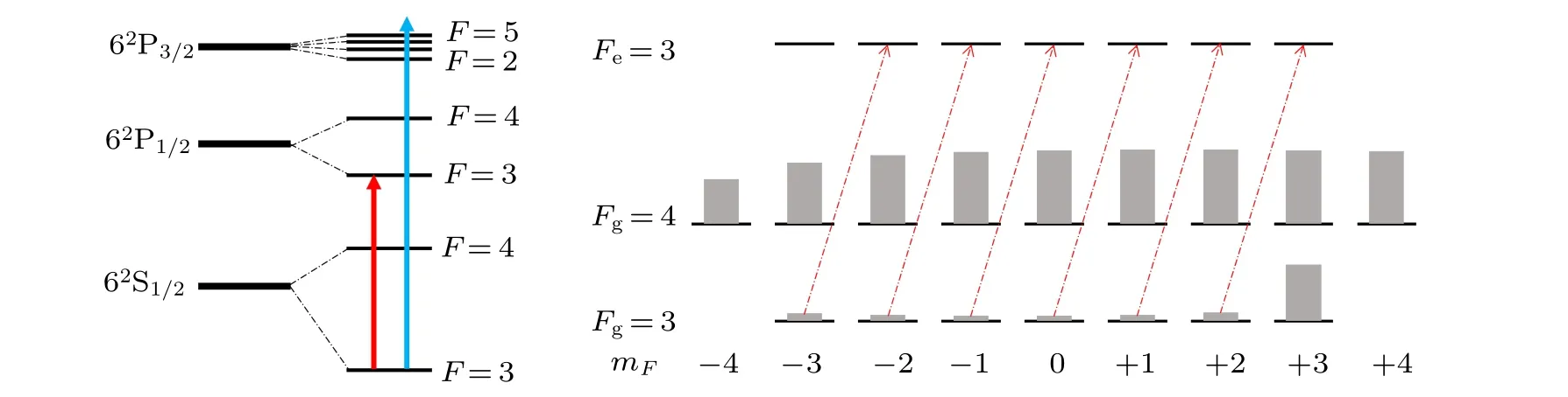
Fig.2. On the left are the energy levels of Cs(not to scale). The red arrow refers to the pump light and the blue arrow refers to the probe light.On the right is the steady-state atomic population in each Zeeman sublevel under experimental conditions. Orientation(κ =1 polarization)is generated in both hyperfine levels.

The core of the system is a Cs atomic vapor cell immersed in the static magnetic field, located at the center of the magnetic shield. The cylinder cell (diameter =2.5 cm,length =2.5 cm) is coated with paraffin inside to moderate the relaxation rate of atomic spin polarization (2π×3.0 Hz for Fg=3 and 2π×1.5 Hz for Fg=4, the difference comes from the spin-exchange collisions[15]). The temperature in the shield is ～22°C and the atomic density in the cell is n ≈3.5×1010atoms/cm3. The shielding factor of the 7-layer magnetic shield (produced by Beijing Zero-Magnet Technology Co., Ltd)is about 10−5. The static magnetic field within the shield is generated by a set of Helmholtz coils(the yellow ring within the shield in Fig.1)driven with a constant current source(Krohn-hite Model 523 calibrator). In our system, the applied magnetic field is B0=5772.7 nT along±ˆz,perpendicular to the propagation directions of the pump beam(−ˆx)and probe beam(−ˆy).

The timing plot is listed in the blue shaded area in Fig.1.There are mainly 3 stages in acquiring the frequency information–polarizing the spins,acquisiting the data,and analyzing the data. It cost 1 s to polarize the atomic spins in both hyperfine levels. In this stage, the pump light(red thick line)is turned on and has its amplitude modulated at the Larmor frequency of hyperfine levels F =I+J and F =I −J (0.5 s for each)successively. Later the pump light is turned off,and the spin polarization in both hyperfine levels will decay at respective relaxation rates. The optical FID signal detected by the polarimetry system takes the form

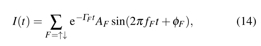
where ΓFis the relaxation rate, fFis the precession frequency of atomic polarization,AFis the amplitude of the polarization,and φFis the phase of the precession. The signal is recorded in the data acquisiting stage. In the last stage, Fourier transform is conducted to the acquisited signal, in order to figure out the precession frequency. The analyzed signal is fitted by the overlapped Lorentzian profiles

where IFand RFare the imaginary and real parts of the magnetic resonance signal. This stage will take 1 s to get the frequency information f↑↓(+). All these stages should be repeated in the inversed magnetic field to acquire the parameterℛ. The total time to get one ℛ data is determined by the acquisition time t for the optical FID signal,which is discussed in the next section.

4. Results and analysis

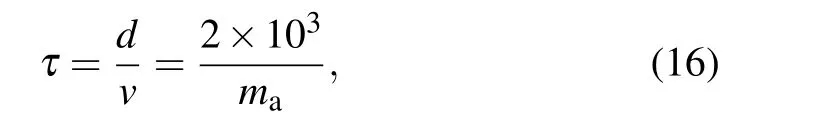
Different with the analysis in detecting spin-gravity interaction[15,21,22]which may persist, to detect the spinaxion-like field couplings which only exist transiently,[1,11,23]the ability to figure out the anomaly transient-in-time signal depends on the duration τ of the transient event,because such parameter determines the intergral time of the signal. For a domain wall with the thickness d,the duration to pass through the earth can be acquired via Eq.(2)

and the resolution of the single-species comagnetometer for the transient event is approximated

where δℛ is the noise spectrum density (sensitivity) of the parameter ℛ with the dimension of Hz−1/2. Comparing Eqs.(13)and(17),we find the sensitivity of the single-species Cs comagnetometer to the coupling constant of proton fpto be

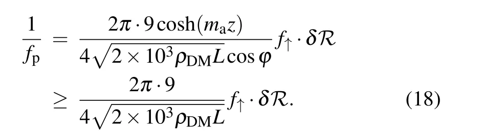
According to the definition of the parameter ℛ in Eq. (12), the sensitivity δℛ is dependent on the sensitivities of the four measured frequencies

Considering the fact that the spin-magnetic interactions are much stronger than exotic spin-dependent interactions,we assume fF(+)≈fF(−)≈γFB. Besides, the sensitivity of frequency is determined by the systematic SNR which should not change when the magnetic field is inversed,and therefore δ fF(+)≈δ fF(−). Taking these assumptions into Eqs. (13)and(19),the systematic sensitivity to couplings between ALPs and proton spin is Given that the optical FID signals are recorded and utlized in our experiments,the estimation of the frequency sensitivity δ f is conducted differently with other magnetometers whose signal amplitude does not decay. To figure out the optimal acquisition time t for better sensitivity of searching for the domain walls,we measured the dependence of the noise spectral density of the parameter ℛ on the acquisition time for optical FID signal t. As shown in Fig. 3(a), when the acquisition time is no more than 500 ms,the δℛ deteriorates obviously with the decrease of the acquisition time. When the acquisition time is more than 600 ms,δℛ is below 2×10−6Hz−1/2.

Fig. 3. (a) The dependence of the noise spectral density of the parameter ℛ on the acquisition time for each optical FID signal. (b) The measured ℛ and(c)the noise spectrum density(sensitivity)δℛ of 2000 consecutive measurements(about 10000 s in total)when the magnetic field is B0=5772.7 nT and the acquisition time t=600 ms.

Furthermore, the mass range of ALPs that the comagnetometer system can search for is determined by the bandwidth,in other word, the total time to get one ℛ data. According to the timing plot in Fig.1,we need to spend ttotal=4+2t in getting one comagnetometer data ℛ,which means the Cs atomic comagnetometer system can only respond to domain walls whose crossing duration τ ≥2ttotalaccording to the Nyquist theorem. Substituting it into Eq. (16), the upper limit on the mass of the ALPs can be calculated as

To broaden the upper limit of the detectable mass range of ALPs while maintaining a good sensitivity,the acquisition time for the optical FID signal is t =600 ms in our system,with the total time to get one ℛ data of ttotal=5.2 s, and the corresponding upper limit of the ALPs mass can be calculated by Eq.(21)as

The lower limit is set by the assumption that the time interval of adjacent domain wall crossings should be no more than 1 year(365×86400 s),and the corresponding mass limit is

To test the performance of the single-species Cs atomic comagnetometer in search for exotic spin-dependent couplings,we run the experimental system for 2000 times successively. The results for parameter ℛ are exhibited in Fig.3(b),and the noise spectral density δℛ is shown in Fig. 3(c). The average value of ℛ deviates about −3×10−7from 0, which may be caused by the light shift induced by the linearly polarized probe beam. Furthermore, the drift of the probe light frequency should be responsible for the fluctuation of measured ℛ in the same way. Such a deviation and fluctuation could be effectively reduced and eliminated by appropriately setting and stabilizing the laser frequency.[22]

which means that ALPs with proton coupling fp3.71×107GeV could be excluded based on the current sensitivity.

The current excluding constraints are below the astrophysical constraints for nucleons as fN109GeV,[5]and the range of ALPs mass is only a small part of the parameter space not excluded by previous constraints. Therefore, to set more stringent constraints on couplings between proton spin and ALPs with a wider range of mass, we need to optimize both sensitivity and bandwidth of our comagnetometer.

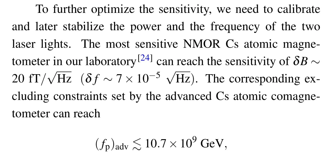
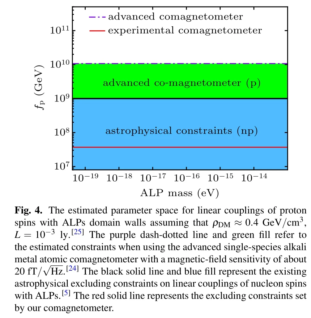
which is one order in magnitude more stringent than existing excluding constraints on the couplings between ALPs and proton spin. These constraints are shown in Fig.4.

To optimize the bandwidth,we need to cut down the time to get one ℛ data. The data processing can be executed in the background and takes no time in the operation sequence of the comagnetometer. Besides, the time consumed in polarizing the atomic spin can be cut down by adding another laser tuned to the center of the Doppler broadened Cs D1 transition in Fg=4 →Fe=4, similar to the double-pump scheme in Ref. [25]. In the stage of polarizing the spins, the two pump lights have their amplitudes modulated at the Larmor frequencies of two hyperfine levels F=3&4 respectively for 0.5 s in total. Furthermore,the two hyperfine levels will have a better orientation(κ =1 atomic polarization),thus better systematic SNR,compared to those in the single-pump scheme.

If these improvements are implemented, then the total time to obtain one ℛ can be as short as 2×(0.5+0.6)=2.2 s,and therefore the bandwidth is optimized to 0.227 Hz. The corresponding upper limit on ALPs mass is ma≤2.99×10−13eV. The lower limit on ALPs mass is dependent on the total running time of the system.

5. Conclusions and outlook

In this work,we present a scheme to search for 2D topological dark matter(the domain wall)via the linear couplings between proton spin and the pseudoscalar field of axion-like particles using a single-species atomic comagnetometer.[15,22]The shift on the precession frequency of atomic spin polarization induced by domain wall crossings is different for atoms in ground-state hyperfine levels due to different contributions from nuclear spin. For alkali metal atoms, it is the single valence proton that dominates the nuclear spin in the nuclear-shell model. By measuring the two precession frequencies of two hyperfine levels in magnetic fields with the same amplitude and opposite directions, the coupling constant between proton spin and axion-like particles can be deduced. For a single-species Cs atomic comagnetometer based on nonlinear magneto-optic rotation which obtains the frequency information from optical free induction decay signal, domain walls with axion-like particle mass ranging within 4.17×10−20eV ＜ma＜1.26×10−13eV can be detected, and the excluding constraints on proton-axion-like field couplings derived from the experimental results can reach fp3.71×107GeV. Single-species Cs atomic comagnetometer has the potential to set more stringent constraints as(fp)lim10.7×109GeV if the systematic signal-to-noise ratio is optimized.[24]

Measures can be taken to optimize the comagnetometer system. The two-pump scheme[25]can be applied to halve the time spend in polarizing the atomic spin and increase the atomic polarization in both hyperfine levels,and the data processing can be done in the background. These may help to broaden the upper limit on the axion-like particles to ma≤2.99×10−13eV. Meanwhile, the frequency of the probe light should be stablized to avoid the deviation of the measured ℛ. Compared with the atomic magnetometers which are currently running in the GNOME,[1,11,12]which suppress the coupling between the electron and ALPs by passive magnetic shielding systems,[14]our single-species atomic comagnetometer has suppressed coupling between the electron and ALPs, and in turn could provide a reliable reference for the science run, data processing,[13]and noise monitoring of the GNOME project.