Markus Enekvist,Xiaodong Liang,Xiangping Zhang,Kim Dam-Johansen,Georgios M.Kontogeorgis,,*

1 Center for Energy Resources Engineering (CERE),Department of Chemical and Biochemical Engineering,Technical University of Denmark,Building 229,Søltofts Plads 229,DK-2800 Kgs.Lyngby,Denmark

2 Hempel Foundation Coatings Science and Technology Centre (CoaST),Department of Chemical and Biochemical Engineering,Technical University of Denmark,Building 229,Søltofts Plads 229,DK-2800 Kgs.Lyngby,Denmark

3 Sino-Danish Center for Education and Research (SDC),IPE,University of Chinese Academy of Sciences,Beijing 100049,China

4 Beijing Key Laboratory of Ionic Liquids Clean Process,CAS Key Laboratory of Green Process and Engineering,State Key Laboratory of Multiphase Complex Systems,Institute of Process Engineering,Chinese Academy of Sciences,Beijing 100190,China

Keywords:Hansen solubility parameters Group contribution method Organic pigments Computer-aided product design Parameter estimation Uncertainty analysis

ABSTRACT The Hansen solubility parameters(HSP)are frequently used for solvent selection and characterization of polymers,and are directly related to the suspension behavior of pigments in solvent mixtures.The performance of currently available group contribution(GC)methods for HSP were evaluated and found to be insufficient for computer-aided product design(CAPD)of paints and coatings.A revised and,for this purpose,improved GC method is presented for estimating HSP of organic compounds,intended for organic pigments.Due to the significant limitations of GC methods,an uncertainty analysis and parameter confidence intervals are provided in order to better quantify the estimation accuracy of the proposed approach.Compared to other applicable GC methods,the prediction error is reduced significantly with average absolute errors of 0.45 MPa1/2,1.35 MPa1/2,and 1.09 MPa1/2 for the partial dispersion(δD ),polar(δP ) and hydrogen-bonding (δH ) solubility parameters respectively for a database of 1106 compounds.The performance for organic pigments is comparable to the overall method performance,with higher average errors for δD and lower average errors for δP and δH .

1.Introduction

Paints and coatings are essential parts of many industries,commonly applied for both surface protection and decorative finishes of various industrial products,buildings,and in the automotive industry.Other notable applications are printing inks,anticorrosive,and antifouling coatings [1].An evolving field in paint and coating technology is advanced product formulation,where products with the desired characteristics are designed through a combination of computer-aided tools,experimentation and experience.One of the challenges is the complex nature of coatings,as they commonly consist of a wide range of components including pigments,polymers,solvents and additives [2].With a solvent fraction of up to 50% by volume,efforts have been made to reduce the environmental footprint and usage of organic solvents with a development towards formulation of high solids formulations.Other developments to limit emissions of organic solvents are to move towards other classes of coatings such as water borne and solvent-free systems.While these advances have been effective,solvent borne coatings are still widely used with solvent fractions from less than 20% in high-solid formulations to above 70% in low-solid formulations [3].

Paint development starts with a problem statement.A paint formulation is devised,usually according to earlier successful formulations,and a sample is then created for testing.After testing,the formulation is revised according to the results in comparison to necessary specifications.This cycle is usually repeated and the difference between the paint properties and specifications is reduced with every iteration,as the optimization steps become smaller and smaller with each cycle [3].As the field of chemical formulation design has expanded,there has been an effort to create a systematic framework for the development of paints and coatings [4–6].Many of the advances relate to solvent selection,and to a lesser extent polymer selection and design.A group of components rarely investigated in the context of product design,however,are pigments.This paper will therefore be focused on expanding the methodology for pigment selection in computer-aided product design (CAPD) of paints and coatings,but a similar approach can also be used for other complex organic components in solvent based CAPD,for example dyes or pharmaceutical formulations.For a more detailed review of computer-aided tools and methods used for design of paints and coatings,a recent manuscript by Jhamb et al.[7]is recommended.

One of the pure component properties commonly used for solvents in CAPD is the solubility parameter,where the upper and lower constraints are determined by the other formulation components[5].For solvent-based coating formulation by CAPD,pigments can be treated as one of the active ingredients.As such,they are selected based on their functionality,such as a specified color.The pigments,which are usually added by experience,must then be compatible with additives,the binder,and the solvent mixture.

For pigments,the HSP are directly related to the suspension behavior and relative sedimentation time in a solvent mixture,as well as their affinity for other components such as binders and stabilizers [8,9].

While experimental verification is preferable,the available data for many groups of chemicals is quite scarce and new experiments for a wide selection of candidates might not be feasible.Here,group contribution (GC) methods are suitable as CAPD requires predictive estimations for many different components with relatively low computational power,and predictions only require an algorithm to find the occurrences of groups for any given structure,so a large pool of potential candidates can be evaluated at a low computational cost.GC methods are also suitable for chemical substitution of unwanted compounds given the comparatively high predictive nature of GC methods for structures not included in the original data set,and capability to generate promising candidates for later experimental verification [10,11].GC methods are used when qualitative estimations are needed,such as for generating promising candidates for experimental verification.As GC methods often are less accurate for large,multifunctional molecules,more rigorous and computationally demanding models can be used for verification[11].A prerequisite for including a property estimation method in a CAPD framework is the accuracy of the method for the chemical group it is applied to.Available GC methods in literature will therefore be tested against experimental HSP data of organic pigments to see if the performance is satisfactory,or if a new method should be developed.

The concept of the three dimensional (Hansen) solubility parameters is frequently used in a similar way to the basic rule‘‘like dissolves like”,and has evolved from the Hildebrand solubility parameter[12].While the solubility parameters are commonly used for solvent selection,the applicability is,however,not limited to solvents.It has also found use as a measure of affinity for solid compounds [8]where the parameters represent cohesion rather than solubility.The partial solubility parameters separates the cohesive energy density into dispersion,polar,and hydrogenbonding parameters,which are related to the total solubility parameter,

One application of the solubility parameters is for the selection of components in solvent-based product design[5,13].For the purpose of CAPD the selection criterion is the difference between solubility parameters [8].While the total Hildebrandt solubility parameter can be used as a product design selection criteria for paint components [14]and has several available estimation methods [15,16],it is considered less accurate when compounds have significant contributions from polar or hydrogen-bonding chemical groups [8].Should an estimation of the total solubility parameter be needed,an approximation can be found either by other estimation methods,or by Eq.(1) using acquired partial solubility parameter values and confidence intervals.

2.Group-contribution Methods for Estimating Solubility Parameters

2.1.Currently available group-contribution methods

Early methods to estimate the Hansen partial solubility parameters were developed for polymers by Hoftyzer and van Krevelen[17],and for solvents by Hoy[18].Two modern group contribution methods used for estimating the solubility parameters of complex organic structures have been created by Stefanis and Panayiotou(SP)and Marrero and Gani(MG),both with group contribution values available in open literature [19,20].The SP method is secondorder while the MG method is third-order,with solubility parameters calculated by Eqs.(2) and (3) respectively,shown below.The MG method in this article uses group values by Hukkerikar et al.,[16]as available in the Technical University of Denmark(DTU) property prediction software ProPred [21].

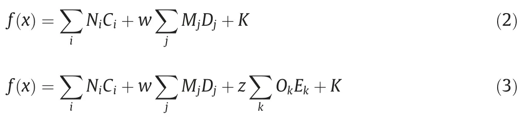
where f（x ）is a function of property x,in this work HSP.Ciis the contribution of group i occurring Nitimes,and Mjis the contribution of group j occurring Djtimes.A universal parameter,K,can be included depending on the method.w can be either 0 or 1 depending on whether the estimation is first-or second-order.The inclusion of z represents the third-order groups k,with Ekoccurrences and a contribution of Ok.The group contributions used for both equations were calculated by two-and three-step regression respectively.

As in other early influential GC methods [22],the first-order groups are basic (UNIFAC) groups to describe the molecular structure.The MG method determines second-order groups from principles that differentiates between isomers and better describes polyfunctional compounds,and third-order groups which describe larger sections of polycyclic compounds [19].For the determination of second-order groups,the SP method follows the principles of conjugation theory,where the groups with the most significant contribution to properties are determined from the most conjugated forms.A more complete theoretical basis for determining the second-order groups is given by the contributions of atoms and bonds to the properties of conjugates [23].Some key points for their selection are,

· Groups based on common conjugation operators should be included in the method as one group.

· Second-order groups can only include adjacent first-order groups,and should not include more groups than necessary.

· The contribution of all second-order groups does not depend on the molecule.

Second-order groups are not included if they are a part of a larger group,but partial overlap of second-order groups is allowed.

2.2.Statistical performance indicators

Evaluation of the regression is based on the following performance indicators [16]:

· The coefficient of determination (R2) provides information on the model fit.An high correlation between experimental data and model estimations is indicated by an R2approaching unity,and is calculated by,

where μ is the mean parameter value.

· The standard deviation (SD) is a measurement of the spread of data around its mean value,calculated from,

· The average absolute deviation (AAD) measures the difference between experimental and predicted values,given by,

· The average relative error(ARE)measures the relative deviation between experimental and predicted values in percent,given by,

2.3.Performance of existing GC methods for organic pigments

Estimations of HSP using the SP and MG group methods are compared to available organic pigment data [24–26],excluding pigments with inorganic elements.Many pigments contain a large number of groups with significant positive or negative contributions to the partial solubility parameters,which in some cases extrapolates to unreasonably high or negative solubility parameter values.The latter is,given the definition as energy density,not possible,as the energy densities cannot be negative,and apolar or non-associating compounds will therefore have parameter values approaching 0 MPa1/2.Fig.1 visualizes the differences between experimental data and the GC estimations as parity plots,excluding negative results.As the estimations differ significantly from experimental data for both the MG method [16]and SP method[20],neither method is appropriate for the purposes of CAPD.There are many possible reasons for this result,such as lack of large multi-functional structures representative of organic pigments in the original regression procedures,or a quantitative or qualitative lack of available data.Table 1 shows the average absolute deviation(AAD) and the average relative error (ARE) for the estimations in Fig.1,calculated according to Eqs.(6) and (7).Pigment structures and calculated HSP are presented in Fig.A1 (Supplementary Material).

3.Method for the Development of a New Group-contribution Method for HSP

The MG method from Hukkerikar et al.[16]uses a total of 220 first-order groups,with a large number of second-and thirdorder groups,which can cause significant parameter identifiability issues for further development due to limitations in the available solubility parameter data.Non-identifiability of parameters is a common problem in regression models,and the estimated group contributions should be determined accurately with low confidence intervals,and uniquely with low linear correlation coefficients between parameters [10,27].The SP method contains fewer groups,and the estimations were more accurate,but was developed with a database limited to solvents and does not include any uncertainty analysis.The accuracy of any estimations using the provided values will therefore be unknown,and extrapolating the method to non-solvents should be avoided.In order to include a more extensive database for parameter regression,and to provide a complete uncertainty analysis,it is therefore considered necessary to develop a new GC method rather than adding new groups while using the available contribution values.The new GC method will be developed based on the SP groups and aims to extend and improve group contribution values for the purpose of predicting the HSP of organic pigments.

3.1.Database

The data used for parameter regression contain a total of 1106 compounds with values for all partial solubility parameters.The data set covers varied and diverse classes of chemicals,including hydrocarbons,solvents,pharmaceuticals,and organic pigments,and was collected from several sources in open literature [8,24–26].The database used for the parameter estimation is included in the Supplementary Material.

3.2.Methodology and parameters

3.3.Maximum likelihood parameter estimation

Fig.1.Parity plot of HSP estimations for organic pigments using the MG method (left) and SP method (right) for δD ,δP ,and δH .

Table 1 Average and absolute errors of group contribution estimations from Fig.1

The GC method to predict the partial solubility parameters of pure components is given by Eq.(2).To find the contributions of Ciand Dj,both simultaneous regression and a two-step regression are performed.Simultaneous regression minimizes the objective function,Eq.(8),for all first-and second-order groups in one regression step,while step-wise regression is performed through sequential parameter estimation of first-order groups and second-order groups separately.

The model parameters,P,are estimated according to the maximum likelihood estimation (MLE) theory by minimizing an objective function,S（P ）,

This objective function is the sum of the squared difference between predicted property values,Xpred,and experimental values,

Xexp,for any given set of parameters [16].N is the total number of components in the database,and j is the evaluated structure.The regression uses weighed least-squares regression and locates the minimum of the objective function with the Levenberg-Marquardt optimization algorithm,which is an iterative search algorithm commonly used for non-linear least-squares problems due to its roboustness and strong convergence properties [28,29].Weighted least-squares regression assume data points with higher variance to be less reliable,and reduces their influence on the objective function by recursively placing high weights on small residuals,and small weights on large residuals [10].

As the experimental data included in the database will contain outliers,which can have a significant detrimental effect on the quality of the GC parameter estimations,it is useful to perform a systematic detection and treatment of outliers.The outliers are detected by an empirical cumulative distribution function (CDF)where the residual values of the estimation are plotted against a step function increasing by 1/N by each measurement.This approach does not depend on normally distributed residuals,which is preferred should the residuals not follow a Gaussian distribution [10].Residuals outside the 95% probability window are treated as outliers,with the dashed lines in Fig.2 indicating the upper and lower 2.5% probability limits.

The methodology for parameter estimation is shown in Fig.3,adapted from Frutiger et al.[10].

3.4.Uncertainty analysis

Given the large differences between predicted solubility parameters and experimental data seen in earlier group contribution methods,it is important to perform an uncertainty analysis for the developed method to know the reliability of estimated data.The analysis is based on the parameter covariance matrix,and assumes the residuals to be independent and to follow a normal distribution with zero mean.The correlation matrices are therefore included in the Supplementary Material.The MLE uses the sum of squared errors (SSE) as given by,

For a linear least squares regression the covariance matrix,COV（P*）,of the estimated model is given by,

where A is the matrix containing occurrences of groups for all structures included in the data set and v is the degrees of freedom(n-p,number of adjustable parameters subtracted from total number of compounds used in the parameter estimation).The error for any given parameter estimation can then be calculated from the linear error propagation,

With the confidence interval(CI)for a property prediction given by,

In Eqs.(11) and (12),t n-p,αt/2

（）refers to the student tdistribution value at（n-p）degrees of freedom at the αt/2 percentile.

Lastly,to test the underlying assumptions it is important to know if the parameters are practically identifiable from the data set.High data availability for a parameter leads to a lower standard deviation,and parameters where the value is identified from few data points will therefore have a greater confidence interval (CI).A high parameter correlation,a measurement of how similar the sensitivity of two parameters are to the model output,suggests that the contribution of one group may depend on the other,meaning the contribution value cannot be estimated uniquely from the data set.A correlation of unity between two parameters means they are completely linearly dependent,and correlations above an absolute value of 0.7 or confidence intervals larger than 50%can indicate poor parameter identifiability [10,30].

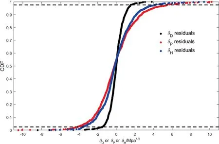
Fig.2.Empirical CDF of residuals in MPa1/2 for δD ,δP ,and δH from parameter estimation using simultaneous weighted least squares regression.The dashed lines represent the upper and lower 2.5% probability window for residuals.

Fig.3.Workflow for parameter estimation for development of the GC method.

4.Method Performance and Discussion for Solubility Parameter Estimations

4.1.Simultaneous regression

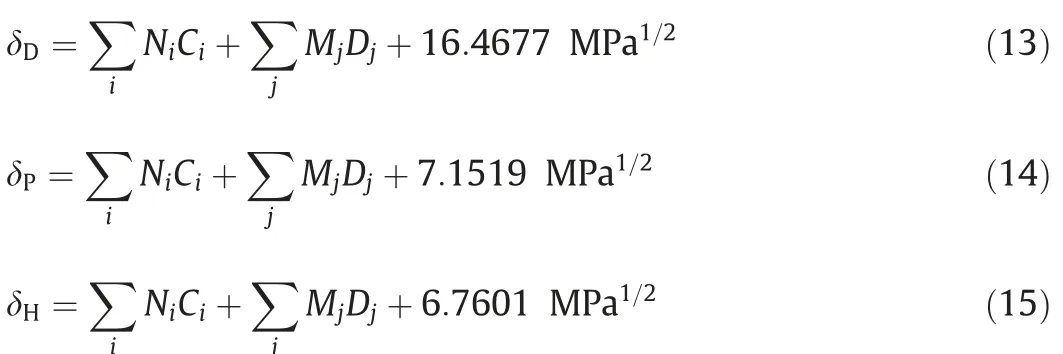
Parity plots visualizing the result of the simultaneous regression are shown in Fig.4,and key performance indicators are presented in Table 2.Eqs.(13)–(15) are used to estimate the HSP,as a sum of the universal parameter and first-and second-order contributions for each occurring group.The contributions are given in Supplementary Material,which also contain the 95% CI for each parameter.

Supplementary Material presents the first-order and secondorder group contributions and the 95%CI obtained from simultaneous regression.

4.2.Step-wise regression

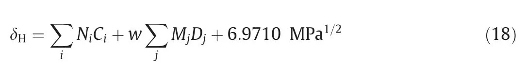
Parity plots visualizing the result of the step-wise regression are shown in Fig.5.Eqs.(16)–(18) are used for estimating the HSP together with the contributions given in Section 2 of Supplementary Material together with the 95% CI.Unlike the simultaneous regression,these equations include the additional parameter w,which can either be set to zero or unity depending on whether second-order groups are included or not in the estimations.

Fig.4.Predicted versus experimental solubility parameter values after outlier treatment using simultaneous regression for δD ,δP ,and δH .Values are in MPa1/2.

Table 2 Key performance indicators of the developed GC regression methods from a total of 1106 compounds

4.3.Regression performance indicators

The performance indicators in Table 2 show that the result is very similar between the different regression methods for the dispersion and hydrogen-bonding parameters,δDand δH,with a slightly larger performance difference between the two regression methods for the polar solubility parameter δP.The different number of data points in Table 2 for each partial solubility parameter is due to the exclusion of apolar and non-associating compounds.Compared to the third-order MG method developed for HSP by Hukkerikar et al.[16]both presented regression methods give higher R2,lower standard deviations,and lower average absolute errors,as shown in Fig.6.The comparison given is for presented performance indicators for the data sets included in each respective method.As the database by Stefanis and Panayiotou [20]is limited to organic solvents it provides lower average absolute errors for the included data,and might be preferable for estimating the HSP of small organic solvents,though the prediction confidence is unknown.The underlying data set for the presented method includes both solvents and non-solvents over a wide space of chemical families to present a more general method,but care should always be taken when extrapolating the values to new molecules.

Notably the average relative error (ARE) is quite large for the polar and hydrogen-bonding parameters.This is not unreasonable for these parameters,as a significant section of the database contains low values and the objective function,Eq.(8),minimizes the absolute error.If the method is applied to compounds with a high polar or hydrogen-bonding energy density the relative error is significantly lower,while the relative error for hydrocarbons is expected to be high.

Fig.5.Predicted versus experimental solubility parameter values after outlier treatment using step-wise regression for δD ,δP ,and δH .Values are in MPa1/2.

4.4.HSP estimation examples for complex pigments with known solubility parameters

in the investigated compound are between the universal constant,ACH,and AC,groups which implies that the groups in question frequently occur at the same time.Full correlation matrices for all groups are presented in the Supplementary Material.

4.5.Method performance for included organic pigment data

As the primary intended application of the developed GC method is to estimate the solubility parameters of various organic pigments,it is of interest to compare its performance to available data.Historically,estimation methods have been known to perform poorly for compounds that are,among other things,(1) solid at room temperature (2) of high molecular weight and (3) polyfunctional [31].These factors apply to organic pigments and are further complicated as the comparison data could be measured in different crystalline states and may be influenced by surface modifications and manufacturing methods.Available experimental data used for comparison does not include organic pigments with inorganic elements,such as metal salt pigments,or measurements where the chemical structure could not be determined[9,24,26,32].

Table 3 provides examples of occurring first-and second-order groups in two selected organic pigments as well as their contribution to each partial solubility parameter.The 95%CI is given by Eq.(12)using a student t-distribution with（n-p）degrees of freedom by subtracting the number of adjustable parameters from the number of data points for each partial solubility parameter [10].

To test the underlying assumptions for the uncertainty analysis,a correlation matrix is presented in Table 4.No correlations are above an absolute value of 0.7,which is the indicator for poor parameter identifiability.The largest linear correlations for groups

To evaluate the performance of the newly developed GC method in predicting solubility parameters of organic pigments,the included pigment data [24–26]is compared to the output of the method.Apart from the method prediction error there are several factors which may influence accuracy.The measured solubility parameters depend on the parameter calculation method [8]and the measurement method [33].In addition to these factors,the functionality of organic pigments differ between different manufacturers and any surface treatment can drastically change surface properties such as solubility parameters [3].

Figs.7–9 show parity plots between predicted and measured δD,δP,and δH,and the direct comparisons including the 95%CI are also presented in the Supplementary Material.Notably,the performance of the different regression methods is very similar,with a few distinct outliers for each partial solubility parameters.Following the regression methodology in Fig.3,clear outliers for either method will not be included in the in the regression step.

Fig.6.Comparison between the R2,SD,and AAD of the developed GC method and presented performance indicators of earlier methods for δD (top left),δP (top right),and δH (center).

Parity plots in Fig.7 reveal two clear outliers with several of the estimations outside of the calculated confidence interval,which is comparatively low relative to the other partial solubility parameters.Excluding two outliers the average relative errors are 4.8%and 4.6%,with average absolute errors of 0.93 MPa1/2and 0.90 MPa1/2for each regression method respectively.The δDestimations are therefore less accurate for included pigments than expected from the overall method performance even excluding the two outliers,possibly due to measurement accuracy of organic pigments.This difficulty can be exemplified by two measurements of the same compound in Supplementary Material,yielding one result above the calculated 95% CI and one result below,as more accurate measurements of other chemical groups provides comparatively low estimation errors.Notably,the measured δDof the two outliers lies outside the range of any other measurements included in the database,while the estimations are close to the other pigment data.

The parity plots in Fig.8 reveal one outlier for the included pigments in the step-wise regression method,which is likely caused by the regression method given the low error given by simultaneous regression.While some relative errors appear high,such as a 59%deviation for Pigment Red 146 using simultaneous regression,this difference is within the 95% confidence interval and is due to the low polarity of the compound.The average relative errors are 12% and 7%,and average absolute errors are 0.81 MPa1/2and 0.63 MPa1/2for each regression method respectively excluding one outlier.The δPestimations are noticeably more accurate than expected from the overall method performance.

A comparison between the estimated and experimentally determined δHyields two outliers significantly outside the calculated 95% CI.Excluding these two outliers,the average relative errors for the estimation of δHare 9% and 8%,and the average absolute errors are 0.77 MPa1/2and 0.67 MPa1/2for each regression method respectively.The estimations of δHfor organic pigments are better than expected from the method performance indicators,however,including outliers the errors are close to the overall method performance.Notably,both outliers are monoazo pigments,which could indicate a poor method performance for this group of pigments,or the experimental data could be influenced by measurement errors,surface treatments,or production differences.It is well known that GC methods are less reliable for large molecules with multiple functional groups [26,31],which could be the cause of larger estimation errors for certain types of pigments,or other chemical groups.To better understand the method accuracy for different groups of pigments,more experimental data for each group would be needed,which could also lower the confidence interval of the estimation as the method performance depends heavily on the included data.

A summary of the performance of the new GC method for estimation of pigment HSP is given in Table 5,which can be compared with estimations from the MG and SP GC methods in Table 1.Some of the issues using earlier methods include too few descriptive second-or third-order groups for the SP method,and a lack of available contribution values for the MG groups due to the large number of first-,second-,and third-order groups.A large number of groups in combination with comparatively low data availability makes the method especially unreliable when applied to large multifunctional compounds like organic pigments.The performance of the SP method for organic pigments is affected by the included database and used groups,which are tailored for the purpose of estimating solvent HSP.These issues are not present in the newly developed GC method,and a detailed uncertainty analysis based on maximum-likelihood estimation (MLE) calculates a confidence interval to better ascertain the accuracy of the estimated parameter for any organic molecule that can be described by the method.The methodology described in this paper can also be usedto more accurately determine group contributions,should data availability increase.

Table 3 Example calculation of Hansen Solubility Parameters using the values from simultaneous regression

Table 4 Parameter correlation matrix example for pigment blue 60,where K is the universal parameter

5.Conclusions

A group contribution method has been developed with the intention of accurately predicting the δD,δP,and δHpartial solubility parameters of organic pigments.The GC model is based on the molecular structure,using first-and second-order groups based on conjugation theory.This method gives a direct estimation of the partial solubility parameter and no experimental data is needed for the predictions.A varied database included in the regression procedure ensures that the groups can estimate solubility parameters of a wide selection of compounds,and inclusion of 95% confidence intervals provides an estimate of the certainty of group contribution parameters and HSP calculations,which depend on the included database.New groups have been introduced to better describe the complex structures of organic pigments,and new group contribution parameters can be used for HSP estimations of both organic pigments and other organic compounds.Outlier treatment,weighted least-squares regression,and an uncertainty analysis provides a more robust method applicable to a wide range of organic molecules.

Fig.7.Parity plot of predicted versus experimental values of δD for organic pigments by simultaneous (left) and step-wise (right) regression.

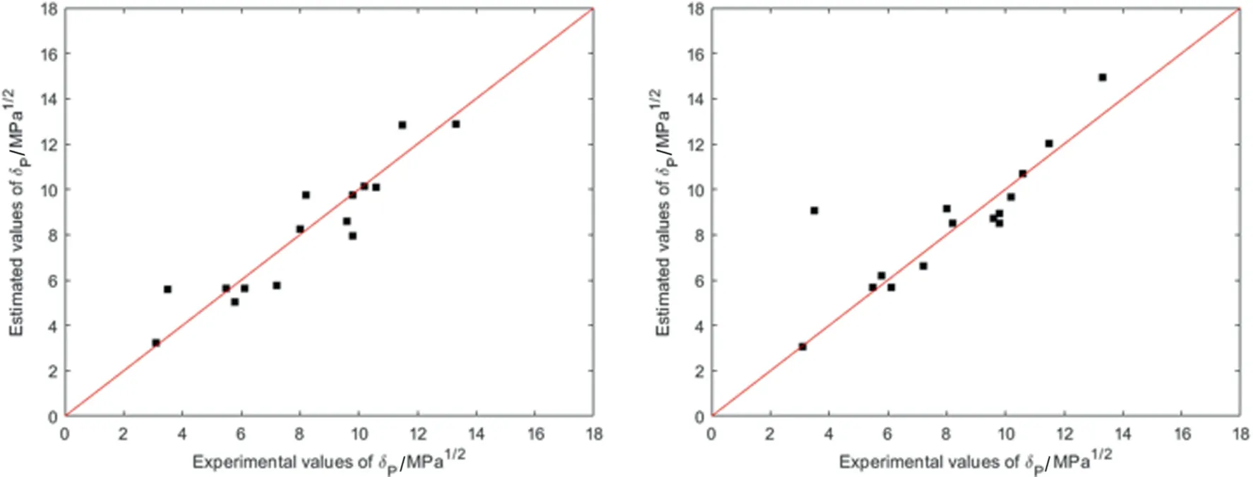
Fig.8.Parity plot of predicted versus experimental values of δP for organic pigments by simultaneous (left) and step-wise (right) regression.

Fig.9.Parity plot of predicted versus experimental values of δH for organic pigments by simultaneous (left) and step-wise (right) regression.

It is clear,in particular for the case of organic pigments,that currently available higher order methods and additional parameters do not inherently increase the accuracy for predicting HSP.The developed model performs well when compared to most available pigment measurements,with some outliers that could be the result of surface treatments,outlier measurements,or failure of GC methods for some complex structures.Estimating the polar partial solubility parameter,δP,has been considered more difficult than the other parameters,which is reflected in the standard deviations and average errors of both regression methods.This difficulty,however,is not reflected in the estimation of pigment solubility parameters,as the results are in good agreement with experimental data.

Table 5 Average and absolute errors of HSP estimations from Figs.7-9 excluding outliers

The developed method can be used for a broad range of applications,including computer-aided product design and solvent selection for complex pure components such as pharmaceuticals,organic dyes,or organic pigments.While the product design process is influenced by many parameters,accurate estimations of pigment HSP could aid in systematic selection of additives like dispersants,or to estimate the compatibility with binders and solvent mixtures.

Declaration of Competing Interest

The authors declare that they have no known competing financial interests or personal relationships that could have appeared to influence the work reported in this paper.

Acknowledgements

Financial support from the Sino-Danish Center for Education and Research(SDC),the Hempel Foundation to CoaST(The Hempel Foundation Coatings Science and Technology Centre),and Hempel A/S is gratefully acknowledged.

Supplementary Material

Supplementary data to this article can be found online at https://doi.org/10.1016/j.cjche.2020.12.013.