THE LOCAL WELL-POSEDNESS OF A CHEMOTAXIS-SHALLOW WATER SYSTEM WITH VACUUM∗
2021-04-12JishanFAN樊继山
Jishan FAN(樊继山)
Department of Applied Mathematics,Nanjing Forestry University,Nanjing 210037,China E-mail:fanjishan@njfu.edu.cn
Fucai LI(栗付才)†
Department of Mathematics,Nanjing University,Nanjing 210093,China E-mail:fli@nju.edu.cn
Gen NAKAMURA
Department of Mathematics,Hokkaido University,Sapporo 060-0810,Japan E-mail:nakamuragenn@gmail.com
Abstract In this paper we prove the local well-posedness of strong solutions to a chemotaxisshallow water system with initial vacuum in a bounded domain Ω⊂R2without the standard compatibility condition for the initial data.This improves some results obtained in[J.Differential Equations 261(2016),6758-6789].
Key words chemotaxis;shallow water;vacuum;local well-posedness;strong solution
1 Introduction
In this paper,we consider the following chemotaxis-shallow water system in Ω×(0,T)(see[1,10]):


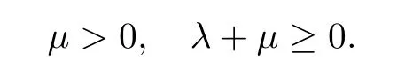
Here ρ,u,n,and p denote the fluid height,the fluid velocity,the bacterial density,and the substrate concentration,respectively.µ and λ are the shear viscosity and the bulk viscosity coefficients of the fluid,respectively,that satisfy the physical condition:
The domain Ω ⊂Ris a bounded domain with smooth boundary ∂Ω,and ν is the unit outward normal vector to ∂Ω.
The system (1.1)–(1.4) can be derived from the chemotaxis-Navier-Stokes equations [10];see [1]for the details.The local well-posedness of strong solutions to the system (1.1)–(1.4)was first obtained by Che et al.[1]under the following compatibility condition for the initial data (ρ,u,n):

for some g ∈L(Ω).Tao and Yao[9]studied the global existence and large time behavior of the solution for the system (1.1)–(1.4) in Runder the condition that the initial data are close to the constant equilibrium.Later,their results were improved by Wang and Wang [11]by using the method of frequency decomposition.Recently,Wang [12]studied the Cauchy problem to a generalized version of the system(1.1)–(1.4)with degenerate viscosity coefficients and obtained the local existence of the unique regular solution with large initial data and a possible initial vacuum.
When n ≡1,(1.1)and (1.2)are reduced to the so-called shallow-water system,while when u ≡0,(1.3) and (1.4) are reduced to the parabolic-parabolic Keller-Segel model.There are many results on these two classical models,and interested readers can refer the references cited in [1].
The aim of this paper is to prove the local well-posedness of strong solutions to the chemotaxis-shallow water system (1.1)–(1.4)with initial vacuum in a bounded domain Ω ⊂Rwithout the assumption(1.7),and hence to improve some results obtained in[1].We will prove

Remark 1.1
Since we used the time weighted energy method,we don’t need to use the compatibility condition (1.7).Moreover,by considering the strong solution in (1.8),we get the existence and uniqueness of strong solutions with less regular initial data.Remark 1.2
For the compressible Navier-Stokes equations,the local well-posedness of strong solutions was obtained by[2,8]under some additional compatibility conditions as follows:
Huang and Li[4]first succeeded in removing the compatibility conditions(1.9)and obtained the existence and uniqueness of local strong solutions for the 2D compressible Navier-Stokes equations.For the Cauchy problem of 2D compressible Navier-Stokes equations,Li and Liang [5]obtained the local well-posdness in unbounded domains without the compatibility conditions(1.9).For the 3D case,it was Huang [3]who first obtained the local well-posdness of compressible Navier-Stokes equations in bounded or unbounded domains without the compatibility conditions (1.9).See Li and Xin [6]for some global well-posedness results on this topic.


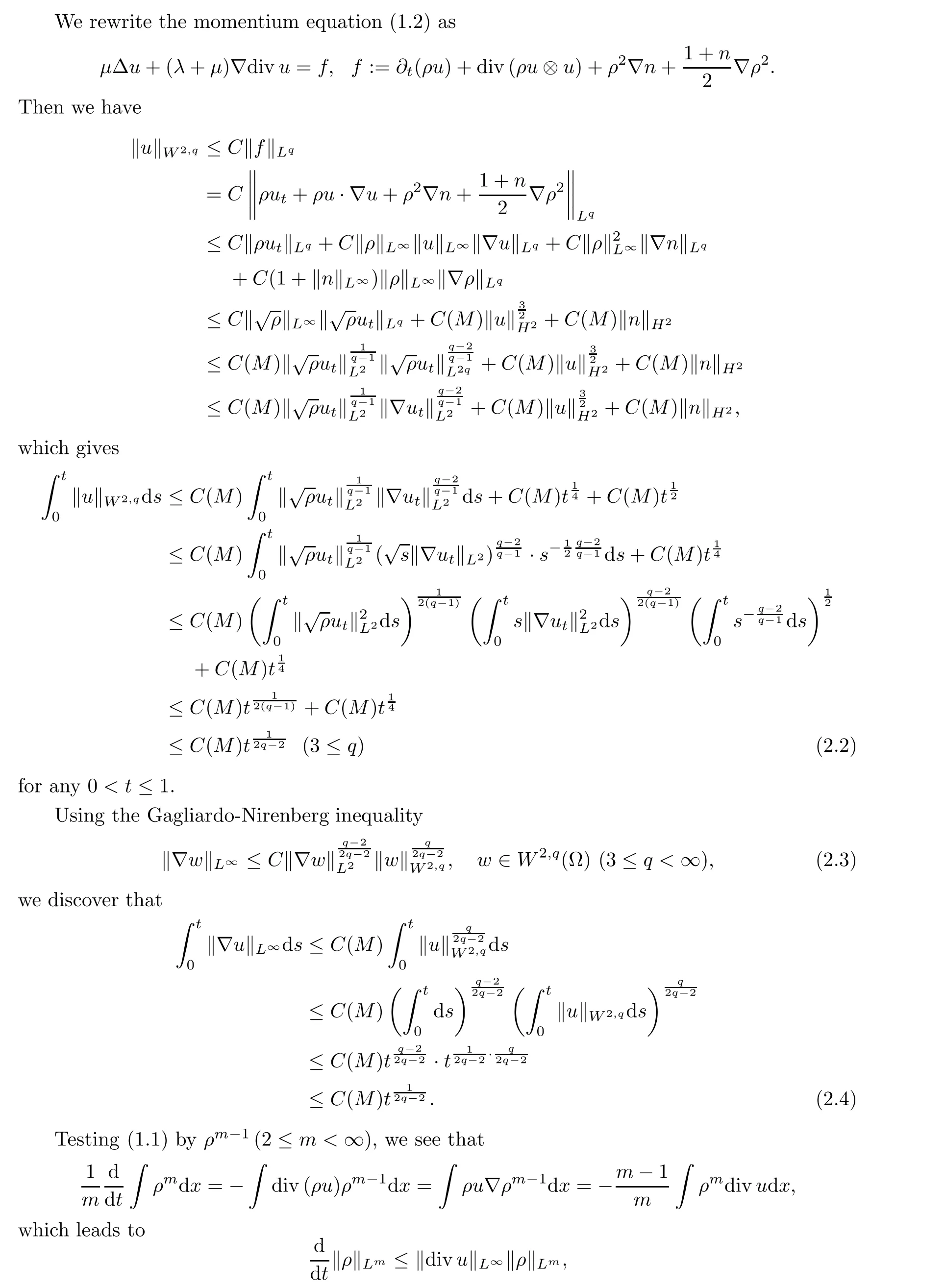
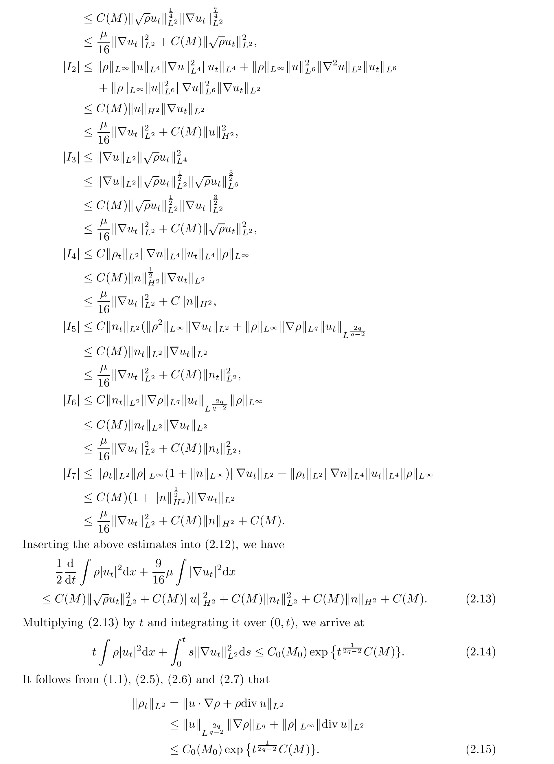
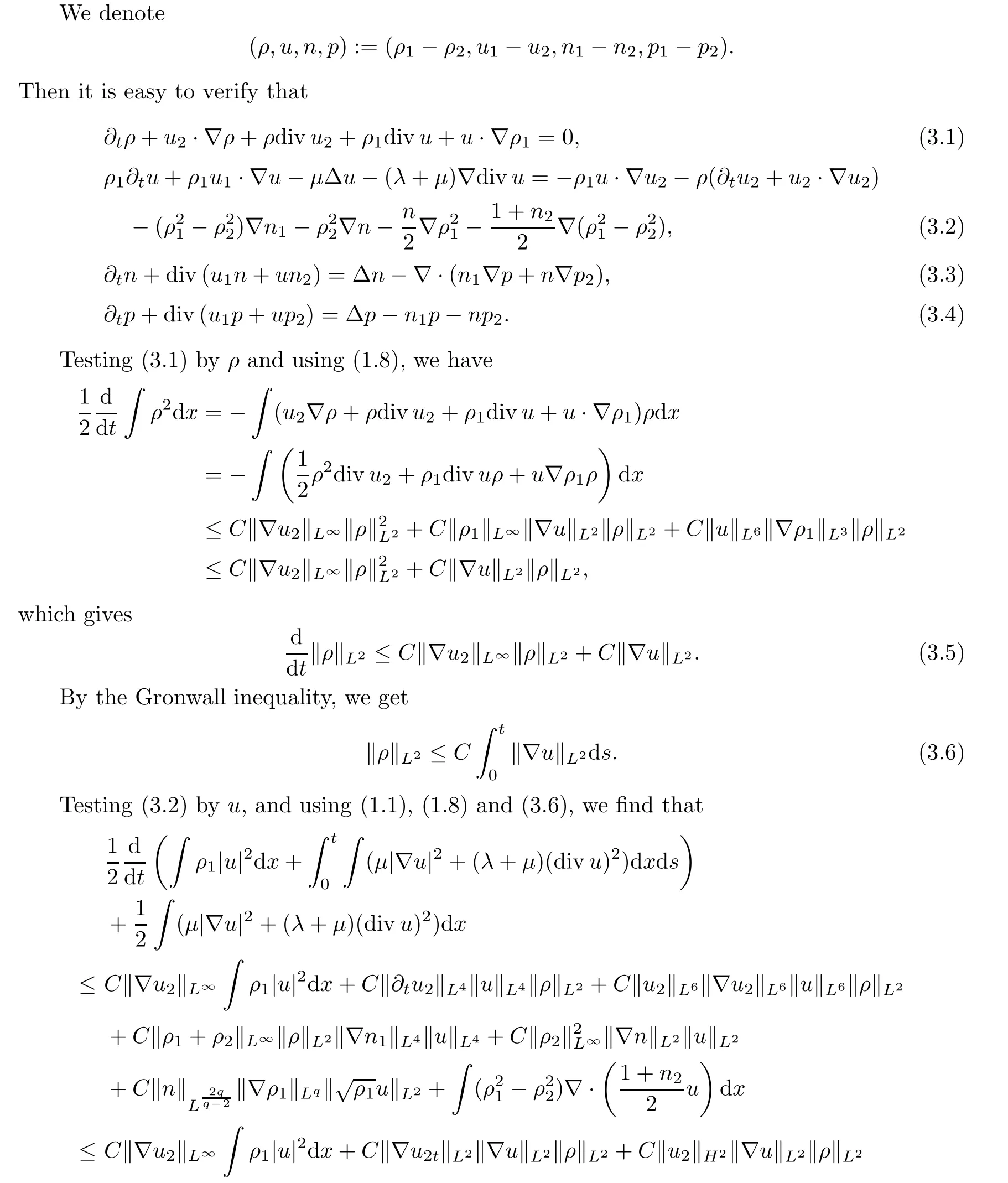
for some constant C >0 on [0,T],where T The remainder of this paper is devoted to the proofs of Theorem 1.2 and the uniqueness part of Theorem 1.1,which are presented in Section 2 and Section 3,respectively. Below,for the sake of simplicity,we shall drop the superscript“δ”of ρ,u,n,pand M.First,thanks to the maximum principle and integration by parts,we see that This section is devoted to the proof of Theorem 1.1.Since the existence part of Theorem 1.1 has been obtained,we now only need to show the uniqueness part.Let (ρ,u,n,p) (i=1,2)be the two strong solutions satisfying (1.8) with the same initial data.2 Proof of Theorem 1.2


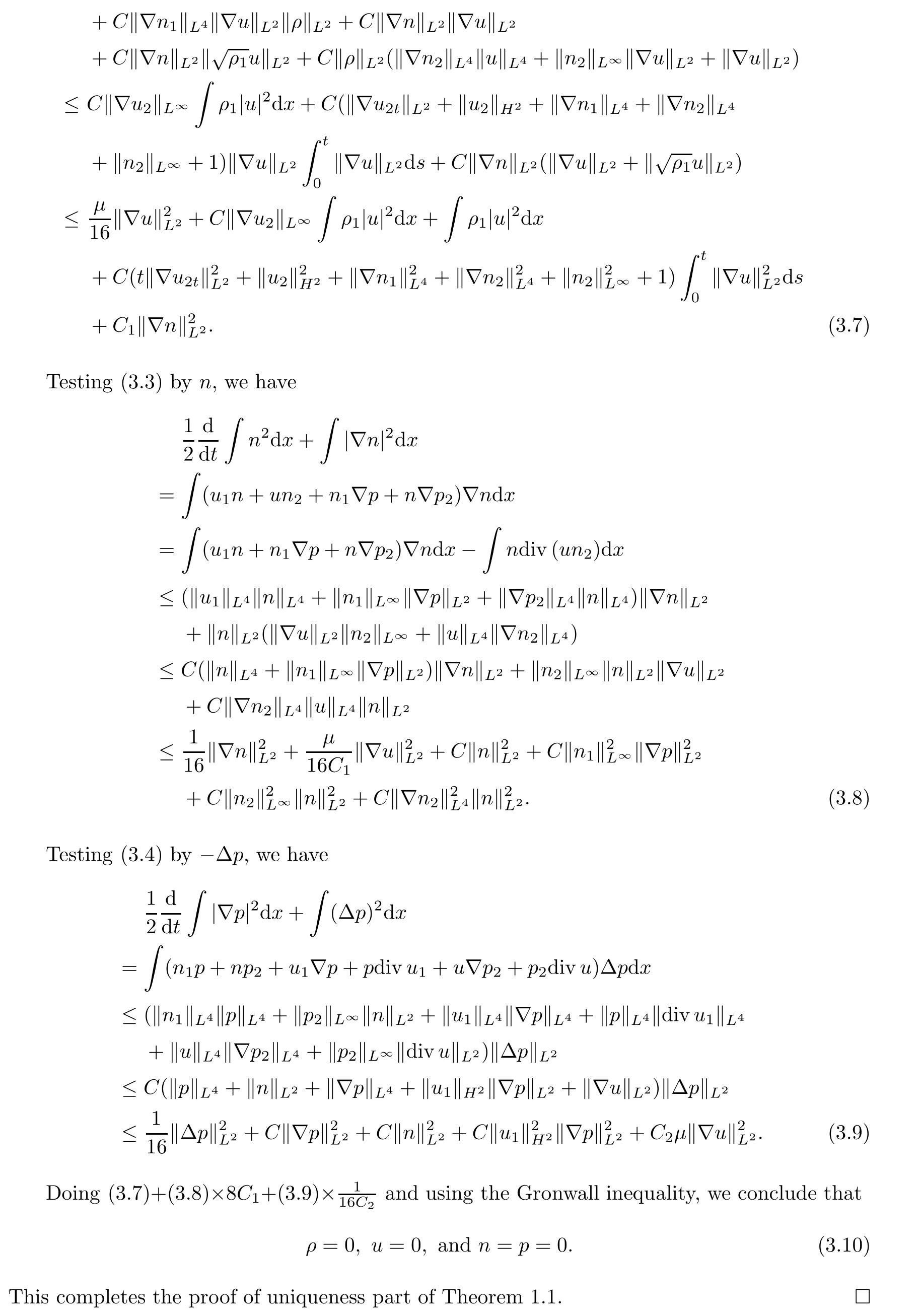
3 Proof of Theorem 1.1
杂志排行

Acta Mathematica Scientia(English Series)的其它文章
- ON THE MIXED RADIAL-ANGULAR INTEGRABILITY OF MARCINKIEWICZ INTEGRALS WITH ROUGH KERNELS∗
- CONTINUOUS DEPENDENCE ON DATA UNDER THE LIPSCHITZ METRIC FOR THE ROTATION-CAMASSA-HOLM EQUATION∗
- WEAK SOLUTION TO THE INCOMPRESSIBLE VISCOUS FLUID AND A THERMOELASTIC PLATE INTERACTION PROBLEM IN 3D∗
- ISOMORPHISMS OF VARIABLE HARDY SPACES ASSOCIATED WITH SCHRÖDINGER OPERATORS∗
- HITTING PROBABILITIES OF WEIGHTED POISSON PROCESSES WITH DIFFERENT INTENSITIES AND THEIR SUBORDINATIONS∗
- INHERITANCE OF DIVISIBILITY FORMS A LARGE SUBALGEBRA∗