Hua CHEN(陈化)

School of Mathematics and Statistics,Wuhan University,Wuhan 430072,China E-mail:chenhua@whu.edu.cn

Nian LIU(刘念)†

School of Science,Wuhan University of Technology,Wuhan 430070,China E-mail:nianliu@whut.edu.cn

Abstract In this article,we study the initial boundary value problem of coupled semi-linear degenerate parabolic equations with a singular potential term on manifolds with corner singularities.Firstly,we introduce the corner type weighted p-Sobolev spaces and the weighted corner type Sobolev inequality,the Poincaré inequality,and the Hardy inequality.Then,by using the potential well method and the inequality mentioned above,we obtain an existence theorem of global solutions with exponential decay and show the blow-up infinite time of solutions for both cases with low initial energy and critical initial energy.Significantly,the relation between the above two phenomena is derived as a sharp condition.Moreover,we show that the global existence also holds for the case of a potential well family.

Key words coupled parabolic equations;totally characteristic degeneracy;singular potentials;asymptotic stability;blow-up

1 Introduction and Main Results

Let M⊂[0,1)×X×[0,1)be a corner type domain withfinite corner measure|M|=which is a local model of stretched corner-manifolds(i.e.,the manifolds with corner singularities)with dimension N=n+2≥3.Here,let X is a closed compact sub-manifold of dimension n emdedded in the unit sphere of Rn+1.Let M0denote the interior of M and∂M={0}×X×{0}denote the boundary of M.The corner-Laplacian is defined as

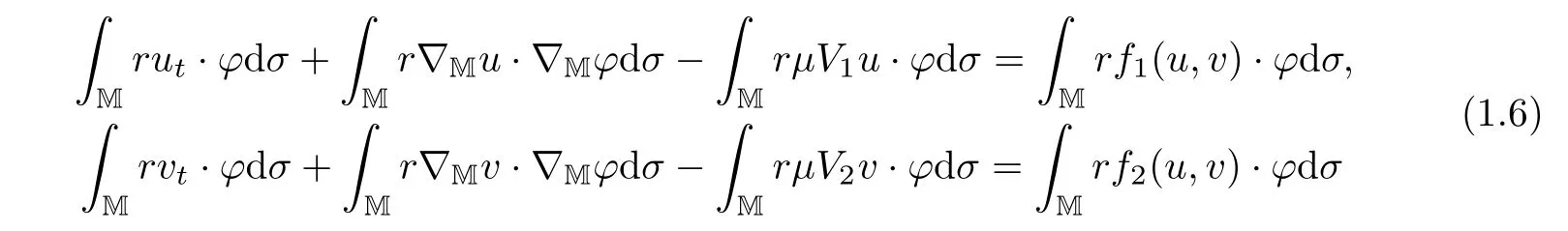
which is a degenerate elliptic operator on the boundary ∂M.The present paper is concerned with the initial boundary value problem of a class of coupled semi-linear corner-degenerate parabolic equations with singular potential term of the form

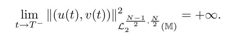
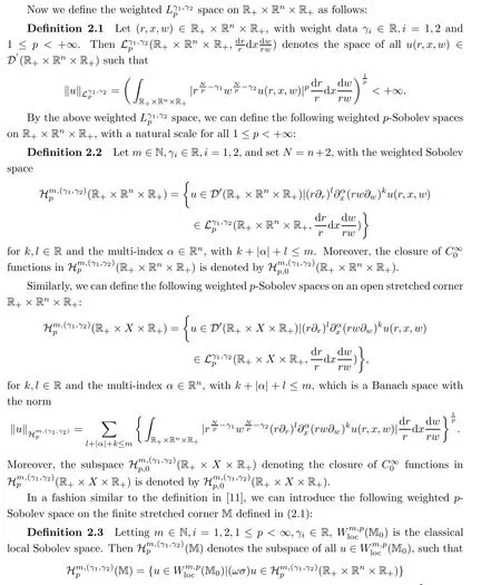
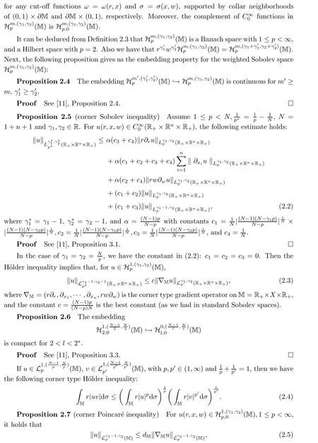
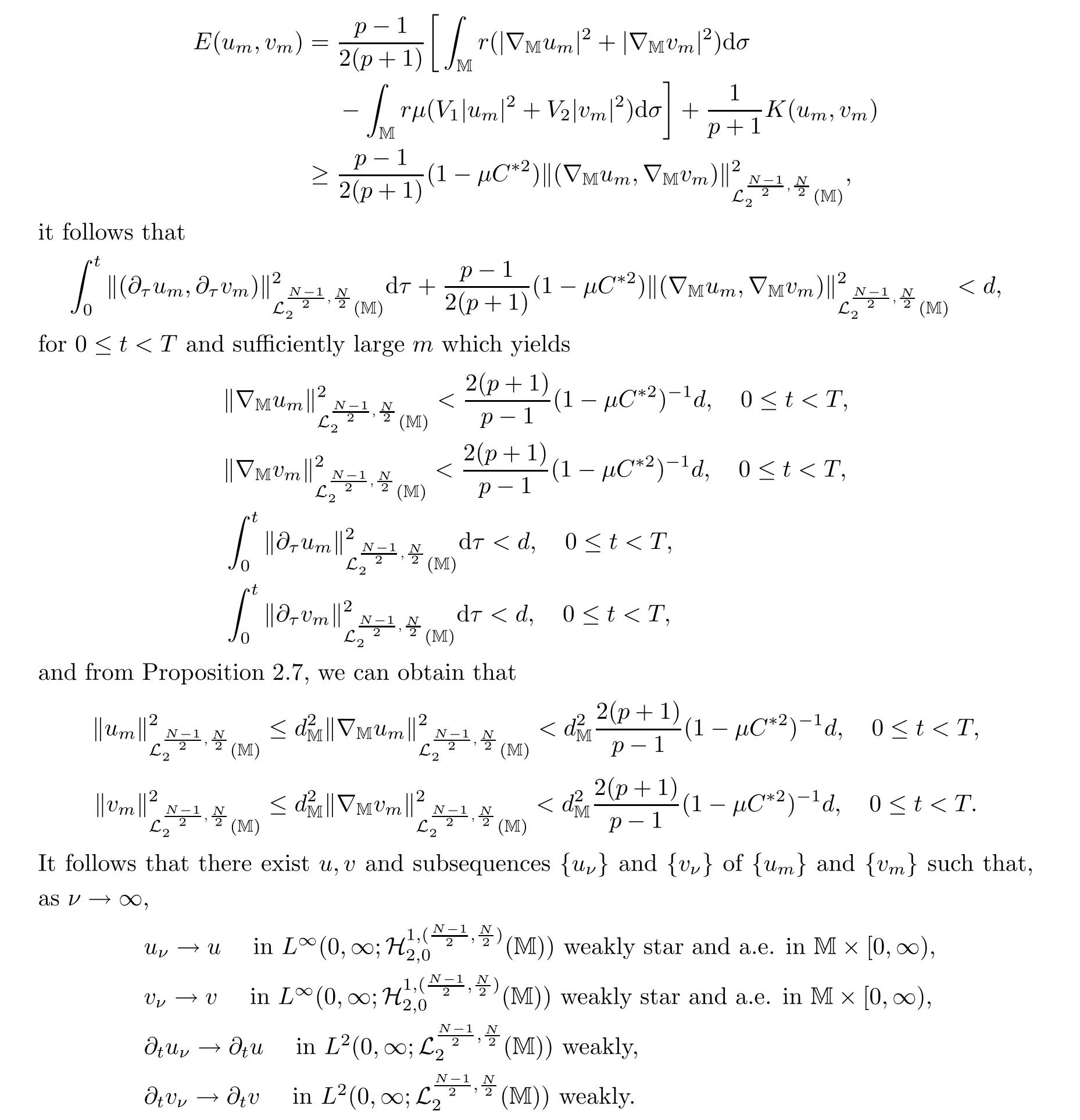
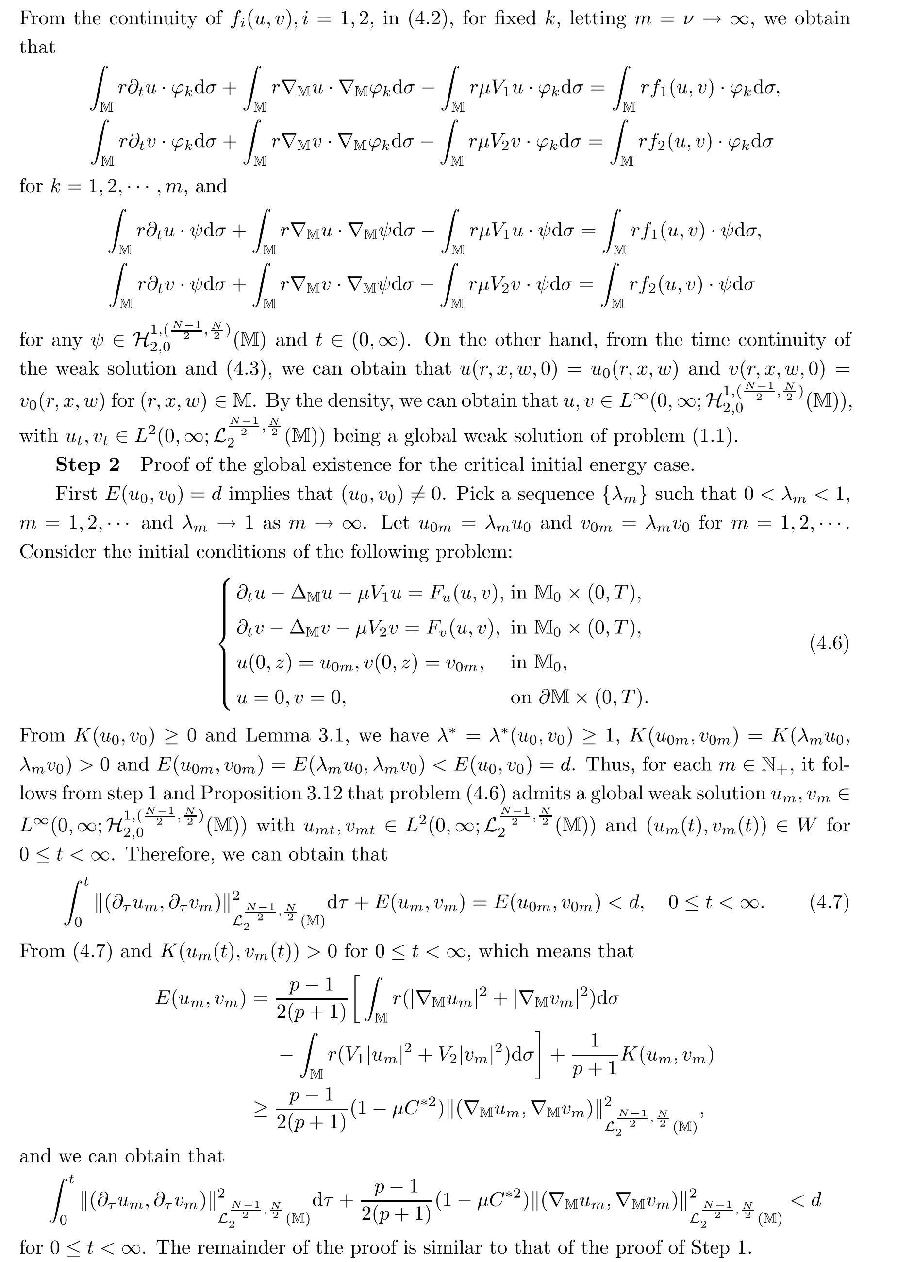
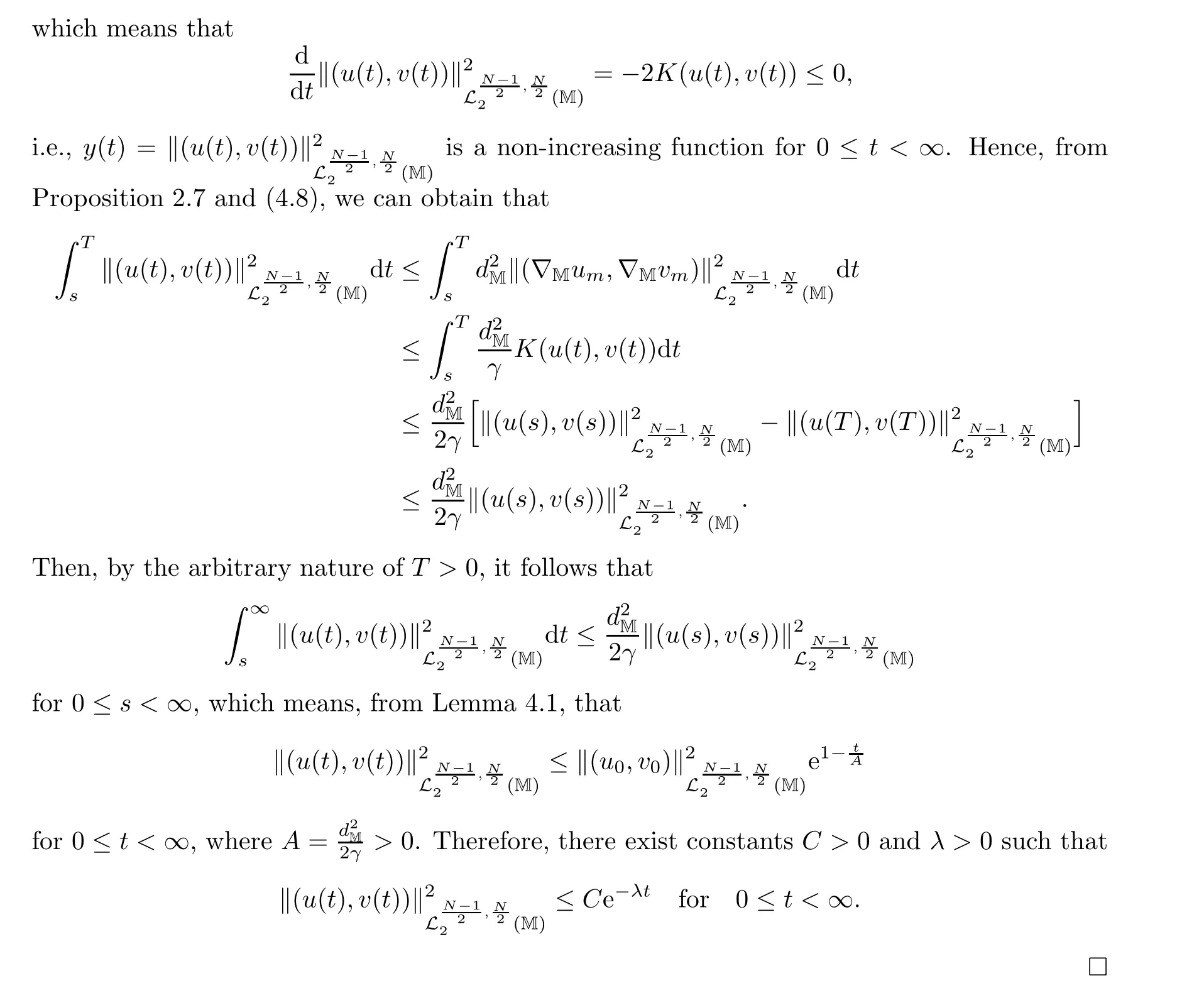
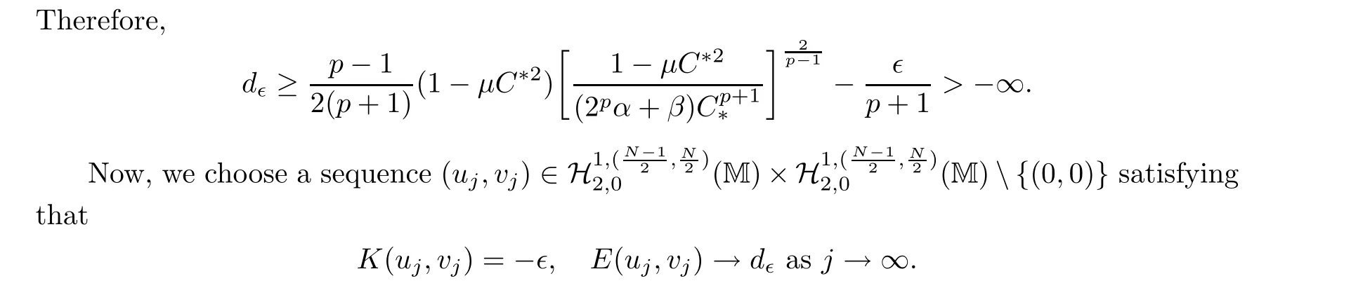
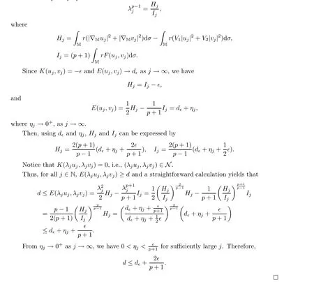
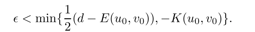
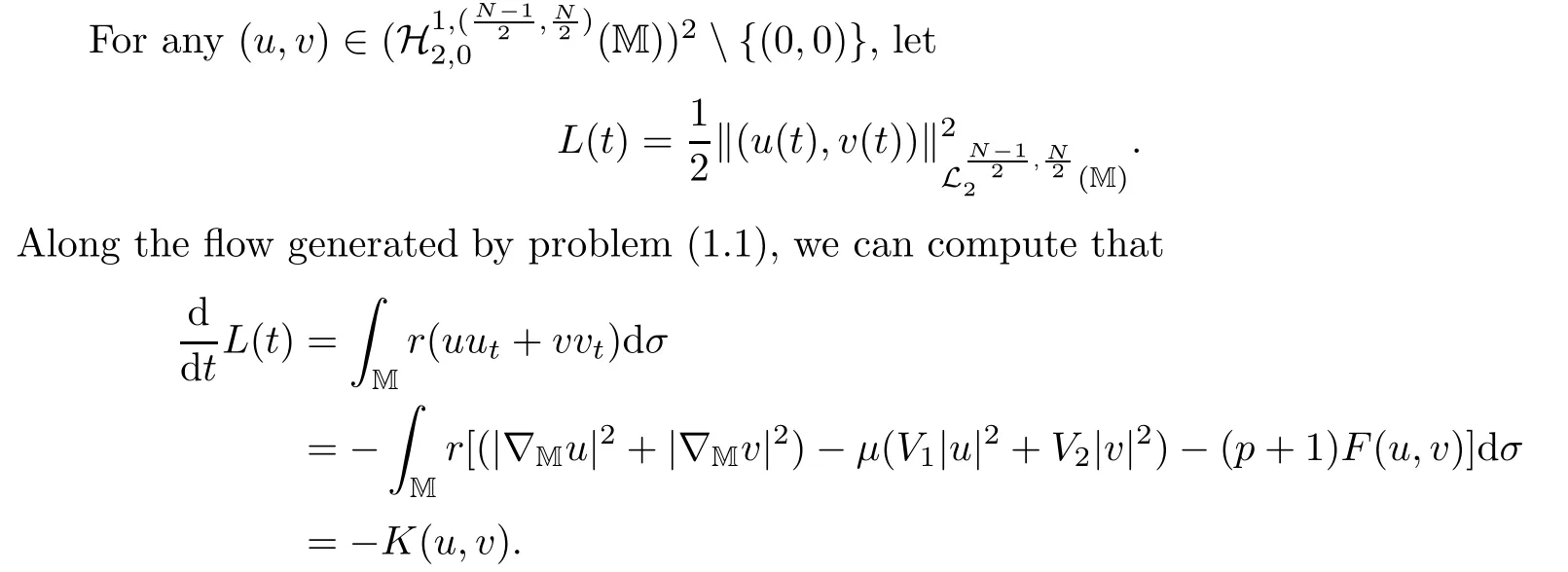
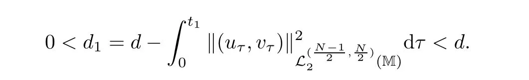
where z :=(r,x,w) ∈M,0

Chen et al.[4]studied the initial-boundary problem of a single semi-linear parabolic equation on a stretched cone.The corresponding cone is Laplacianwhich is degenerate at x1=0.This kind of operator is a simple example of conical dfferential operators.Alimohammady and Kalleji [2]studied a similar problem for a class of single semilinear parabolic equations with a positive potential function on stretched cone.The authors of this paper [3]studied the initial-boundary problem of a single semi-linear parabolic equation with a singular potential function for the edge Laplacian(w∂y1)2+···+(w∂yq)2,with edge singularity at w=0.A powerful technique for treating the above problems is the so-called potential well method,which was developed by Sattinger[21]in the context of hyperbolic equations.At the same time,the pseudo-differential operators with conical singularities and edge singularities have been widely studied with various motivations by Egorov and Schulze [14],Schulze [23],Schrohe and Seiler [22],Melrose and Mendoza [18]and Mazzeo [17],Chen et al.[5–10].

Motivated by the above work,in this article we generalize the above results for scale parabolic equations to a coupled system of nonlinear parabolic equations.We further study a class of coupled systems of semi-linear parabolic equations with singular potentials on a manifold with corner singularities.Here the so-called corner Laplacian ∆M=(r∂r)2+(∂x1)2+···+(∂xn)2+(rw∂w)2is degenerate at both r=0 and w=0,and it is named after the local structure of a manifold with corner singularities.Recently,Chen et al.[11]established the so-called corner type Sobolev inequality and Poincaré inequality in the weighted Sobolev spaces.Such kinds of inequalities will be of fundamental importance in proving the existence of weak solutions for nonlinear problems with corner degeneracy.Melrose and Piazza studied the structure of manifolds with corners in [19].Schulze discussed the calculus of corner degenerate pseudo-dfferential operators in [24].Chen et al.studied multiple solutioms and multiple sign changing solutions for semi-linear corner degenerate elliptic equations with singular potential in [13]and [12],respectively.

First,we introduce the following definition of the weak solution:

Definition 1.1Function (u,v)=(u(z,t),v(z,t)) is called a weak solution of problem (1.1) on M × [0,T),with 0

From the variational point of view,there are two natural functionals onassociated with problem (1.1):the energy functional and the Nehari functional.These are defined respectively,by

Remark 1.2The weak solution in the above definition satisfies the conservation of energy

We are now in a position to state our main results.Our main results are concerned with the global existence with exponential decay and the finite time blow-up of a solution for problem(1.1).Let

Theorem 1.4Let u0,v0∈.Assume that E(u0,v0)≤d and K(u0,v0)≤0.Then the weak solution of problem (1.1) blows up in finite time,i.e.,the maximal existence time T is finite and

This paper is organized as follows:in Section 2 we give some preliminaries,such as the definition of a corner type weighted p-Sobolev space,the properties of corner type weighted p-Sobolev space and some useful inequalities,such as the Sobolev inequality,the Poincaré inequality and the Hardy inequality (more details can be seen in [11,13]).In Section 3,we introduce a family of potential wells relative to problem(1.1)and prove a series of corresponding properties.Then,we discuss the invariance of some sets under the solution flow of (1.1) and the vacuum isolating behavior of solutions.Finally,we give the proof of Theorem 1.3 and Theorem 1.4 in Section 4.Moreover,we show that the global existence also holds for the case of a potential well family.

2 Corner Type Weighted p-Sobolev Spaces

Let X ⊂Snbe a bounded open set in the unit sphere of.Then the finite corner is defined as

where the base E is a finite cone defined as E=([0,1)×X)/({0}×X).Thus,the finite stretched corner is

with the smooth boundary ∂M={0}×X ×{0}.Here we denote M0as the interior of M.In this paper,we shall use the coordinates (r,x,w)∈M.

The typical degenerate differential operator A on the stretched cone E is as follows:

where gXis a Riemannian metric on X.Then the corresponding gradient operator with corner degeneracy is

has a discrete set of positive eigenvalues {λk}k≥1which can be ordered,after counting (finite)multiplicity,as 0 <λ1≤λ2≤λ3≤··· ≤λk≤···,and λk→∞as k →+∞.Also,the corresponding eigenfunctions{ψk}k≥1constitute an orthonormal basis of the Hilbert space

3 A Family of Potential Wells and Vacuum Isolating of Solutions

In this section,we shall introduce a family of potential wells,the exterior of the corresponding potential well sets,and give a series of properties of these.Then,the invariant sets and the vacuum isolating of solutions for problem (1.1) are discussed.First,let the definitions of functionals E(u,v) and K(u,v) be defined by (1.7)and(1.8).Next,we give some properties of the above functionals as follows:

(iii) E(λu,λv) is strictly increasing on 0 ≤λ <λ∗,strictly decreasing on λ >λ∗,and takes the maximum at λ=λ∗;

(iv) K(λu,λv)>0 for 0<λ<λ∗,K(λu,λv)<0 for λ>λ∗and K(λ∗u,λ∗v)=0,which means that λ∗=1.

Thus,the potential well associated with problem (1.1) is the set

Here,d is the depth of the potential well,which is defined by (1.10) and satisfies (3.2).

The exterior of the potential well is the set

Additionally,we show how d(δ) behaves with respect to δ in the following lemma:

Lemma 3.6d(δ) satisfies the following properties :

(ii) d(δ) is increasing on 0 <δ ≤1,decreasing on 1 ≤δ ≤,and takes the maximum d=d(1) at δ=1.

ProofFrom Lemma 3.5,we immediately obtain the result of (i) and we also have that

Lemma 3.7Assume that 0

ProofE(u,v) >0 impliesIf the sign of Kδ(u,v) is changeable for δ ∈(δ1,δ2),we can choose∈(δ1,δ2) satisfyingThus,by the definition of d(δ),we have E(u,v) ≥However,from Lemma 3.6,E(u,v)=d(δ1)=which is a contraction.

After the definition of the depth of the family of potential wells d(δ),the following lemmas are given to exhibit the relation betweend(δ):

Lemma 3.8Let u,v ∈(M) and 0<δ <.Assume that E(u,v)≤d(δ).

From the definition of Wδand Zδand Lemma 3.6 we can obtain

Lemma 3.11The potential well sets and its outsiders have the following properties:

(i) If 0<δ′<δ′′≤1,then Wδ′⊂Wδ′′.

(ii) If 1 ≤δ′<δ′′<,then Zδ′⊂Zδ′′.

Next,by using the above potential wells,we establish the invariant sets and the vacuum isolating of solutions for problem (1.1).

Proposition 3.12Assume that u0,v0∈(M).Let 0<δ <.Suppose that 0 0 belong to Wδfor δ1<δ <δ2.

ProofLet(u(t),v(t)) be any solution of problem(1.1)with E(u0,v0)=e,K(u0,v0)>0,and let T is the maximal existence time of (u(t),v(t)).From Lemma 3.6,it follows that

for δ1<δ <δ2.From Lemma 3.7,it follows that Kδ(u0,v0) >0 for δ1<δ <δ2.Hence,we can obtain that (u0,v0)∈Wδfor δ1<δ <δ2.

Our goal is to prove that (u(t),v(t)) ∈Wδfor t ∈[0,T) and δ1<δ <δ2.We argue by contradiction.Assume that there exist a δ0∈(δ1,δ2) and t0∈(0,T) such that (u(t0),v(t0))/∈Wδ0,which means that E(u(t0),v(t0)) ≥d(δ0) or Kδ0(u(t0),v(t0)) ≤0 and (u(t0),v(t0))(0,0).

If Kδ0(u(t0),v(t0))=0 and (u(t0),v(t0))(0,0),then (u(t0),v(t0)) ∈Nδ0,by the definition of Nδitself.From the definition of d(δ),we can obtain that E(u(t0),v(t0))≥d(δ0).

If Kδ0(u(t0),v(t0)) <0 and (u(t0),v(t0))(0,0),from the time continuity of Kδ(u,v)and Kδ0(u0,v0) >0,we can obtain that there exists at least one s ∈ (0,t0) such that Kδ0(u(s),v(s))=0.Put

Consequently,Kδ0(u(t∗),v(t∗))=0 and Kδ0(u(t),v(t))<0 for t ∈(t∗,t0).

We have two cases to consider:

Case 1(u(t∗),v(t∗))(0,0).In this case,(u(t∗),v(t∗)) ∈Nδ0,by the definition of Nδitself.From the definition of d(δ),we can obtain that E(u(t∗),v(t∗))≥d(δ0).

By recalling the conservation of energy (1.9),we note that

for t ∈[0,T) and δ1<δ <δ2.Hence,E(u(t0),v(t0))≥d(δ) is impossible for any δ1<δ <δ2.

Case 2(u(t∗),v(t∗))=(0,0).In this case,we must have Kδ0(u(t),v(t))<0 for t ∈(t∗,t0).Thus,from Lemma 3.3,we can obtain that

Proposition 3.13Assume that u0,v0∈.Let 0<δ <.Suppose that 0

ProofLet(u(t),v(t)) be any solution of problem(1.1)with E(u0,v0)=e,K(u0,v0)<0,and that T is the maximal existence time of (u(t),v(t)).From Lemma 3.6,it follows that

for δ1<δ <δ2.From Lemma 3.7,it follows that Kδ(u0,v0) <0 for δ1<δ <δ2.Hence,we can obtain that (u0,v0)∈Zδfor δ1<δ <δ2.

Our goal is to prove that (u(t),v(t)) ∈Zδfor t ∈[0,T) and δ1<δ <δ2.We argue by contradiction.Assume that there exist a δ0∈(δ1,δ2) and t0∈(0,T) such that (u(t0),v(t0))/∈Zδ0,which means that E(u(t0),v(t0))≥d(δ0) or Kδ0(u(t0),v(t0))≥0.

If Kδ0(u(t0),v(t0)) ≥0,from the time continuity of Kδ(u,v) and Kδ0(u0,v0) <0,we can obtain that there exists at least one s ∈(0,t0) such that Kδ0(u(s),v(s))=0.Put

Consequently,Kδ0(u(t∗),v(t∗))=0 and Kδ0(u(t),v(t))<0 for t ∈(0,t∗).

We have two cases to consider:

Case 1(u(t∗),v(t∗))(0,0).In this case,(u(t∗),v(t∗)) ∈Nδ0,by the definition of Nδitself.From the definition of d(δ),we can obtain that E(u(t∗),v(t∗))≥d(δ0).

By recalling the conservation of energy (1.9),we note that

for t ∈[0,T) and δ1<δ <δ2.Hence,E(u(t0),v(t0))≥d(δ) is impossible for any δ1<δ <δ2.

Case 2(u(t∗),v(t∗))=(0,0).In this case,we must have Kδ0(u(t),v(t))<0 for t ∈(0,t∗)and(u(t),v(t))=0.Thus,from Lemma 3.3,we can obtain that

for t ∈(0,t∗),which is in contradiction with

The above propositions indicate the invariance of Wδand Zδ,respectively.Moreover,concerning their intersections with respect to δ,we have

Proposition 3.14Assume that u0,v0∈Let 0<δ <.Suppose that 0

are invariant under the flow of problem (1.1),provided that 0

The following proposition shows that between these two invariance manifolds,Wδ1δ2and Zδ1δ2,there exists a so called vacuum region,for which no solution exists:

Proposition 3.15Assume that u0,v0∈.Let 0<δ <.Suppose that 0

Remark 3.16The vacuum region becomes bigger and bigger with the decreasing of e.As the limit case,we obtain

4 Sharp Threshold for Global Existence and Blow-up of Solutions

In this section we prove the main results by making use of the family of potential wells introduced above.First we have the following lemma of Komornik [15],which plays a critical role in the study of the exponential asymptotic behavior for global solutions of problem (1.1):

Lemma 4.1Let y(t):R+→R+be a non-increasing function,and assume that there is a constant A>0 such that

Proof of Theorem 1.3We divide the proof in three steps.

Step 1Proof of the global existence for the low initial energy case.

If E(u0,v0) 0.

By (4.3) we can get E(um(0),vm(0))→E(u0,v0)

Next,we prove that (um(t),vm(t)) ∈W for sufficiently large m and 0 ≤t 0 such that(um(t0),vm(t0))∈∂W.Then E(um(t0),vm(t0))=d or K(um(t0),vm(t0))=0 and(um(t0),vm(t0))(0,0).From(4.5)we can obtain that E(um(t0),vm(t0))d.If K(um(t0),vm(t0))=0 and(um(t0),vm(t0))(0,0),then (um(t0),vm(t0)) ∈N.By the definition of d=inf{E(u,v);(u,v) ∈N},we can obtain that E(um(t0),vm(t0))≥d,which contradicts (4.5).

Hence,from (4.5) and

Step 3Proof of asymptotic behavior.

If E(u0,v0)0,from Proposition 3.12 we can obtain that (u(t),v(t))∈W,i.e.,E(u(t),v(t))0 for 0 ≤t<∞.If E(u0,v0)=d and K(u0,v0)≥0,from the approximative solution (um(t),vm(t))∈W,we can obtain that (u(t),v(t)) ∈¯W,i.e.,E(u(t),v(t))≤d,K(u(t),v(t))≥0 for 0 ≤t<∞.Hence,the definition of C∗implies that

Next,we show that the global existence also holds for the case of potential well family.

Corollary 4.2Let u0,v0∈(M).Assume that E(u0,v0)≤d and Kδ2(u0,v0)≥0,where δ1<δ2are two roots of equation d(δ)=E(u0,v0).Then problem (1.1) admits a global weak solution u,v ∈C(0,∞;(M))with ut,vt∈L2(0,∞;and(u(t),v(t))∈Wδfor δ1<δ <δ2,t ∈[0,∞).

ProofFrom Theorem 1.3 and Proposition 3.12,we note that to prove Corollary 4.2,it is sufficient to show that K(u0,v0) >0,from Kδ2(u0,v0) >0.Indeed,if this is false,then there exists a∈[1,δ2) such thatCombining the fact that (u0,v0)(0,0),because of Kδ2(u0,v0) >0,we get thatHowever,from Lemma 3.6,we have E(u0,v0)=d(δ1)=d(δ2)

Instead of considering the global existence result that depends on K(u0,v0),we study the global existence of problem (1.1) with initial data u0,v0,relying on thenorm.

Moreover,we also can suppose that E(uj,vj) is decreasing.

For each (uj,vj),one can choose a λj∈R such that K(λjuj,λjvj)=0.In fact,λjcan be determined explicitly by

Now we can give the proof of Theorem 1.4.

Proof of Theorem 1.4We divide the proof into two steps.

Step 1Let us first consider the low initial energy case.

If E(u0,v0)

For (u0,v0)∈Z,we choose ǫ>0 such that

From the choice of ǫ,it is obvious that K(u0,v0)<−ǫ.

We claim that K(u(t),v(t)) <−ǫ for all t ∈(0,T),where T >0 is the maximal existence time.Otherwise,from the time continuity of K(u(t),v(t)),there is t1∈(0,T) satisfying K(u(t1),v(t1))=−ǫ.By using Lemma 4.4,we know that

From the conservation of energy (1.9),we have E(u(t),v(t))

Since (u0,v0) ∈Z,from Proposition 3.13 we know that (u(t),v(t)) ∈Z.It follows thatfor t ≥0,i.e.,L(t) is increasing along the flow generated by problem (1.1).

By the claim,we can obtain that=−K(u(t),v(t))>ǫ for any t ∈(0,T).Integrating from 0 to t,we have

From (4.10),we can obtain that L(t) ≥0 for 0

This is a contradiction,since the right-hand side of the above inequality goes to −∞as t →+∞.Therefore,the solution of problem (1.1) blows up in a finite time.

Step 2Now we consider the critical initial energy case.

Let(u(t),v(t)) be a weak solution of the problem(1.1)with E(u0,v0)=d>0,K(u0,v0)<0,and T being the maximal existence time of (u(t),v(t)).Let us prove T <∞.From the time continuity of E(u(t),v(t)) and K(u(t),v(t)),we know that there exists a sufficient small t1∈(0,T) such that E(u(t1),v(t1)) >0 and K(u(t),v(t)) <0 for 0 ≤t ≤t1.Thus we can deduceThereforedτ is strictly increasing for 0 ≤t ≤t1,and we can choose t1such that

Since E(u0,v0)=d,from the conservation of energy (1.9) and the above inequality,we can obtain that

If we take t=t1as the initial time,then E(u(t1),v(t1))