LI Xiangyang,ZHANG Shaohua

(1.BGP Inc.,China National Petroleum Corporation,Zhuozhou 072750,China;2.China University of Petroleum (Beijing),Beijing 102249,China)

Abstract: This paper reviews the use of shear-wave splitting in exploration seismology,how it began and how it has been used to characterize fractured hydrocarbon reservoirs in the past forty years since it was first confirmed in earthquake seismology and subsequently introduced to the hydrocarbon industry.Shear-wave splitting (or birefringence) refers to the phenomenon that when a shear-wave enters a fractured medium,it necessarily splits into a fast and slow wave.The fast wave is usually polarized along the fracture strike,the slow-wave perpendicular to the strike,and the time-delay between the fast and slow wave is proportional to the fracture density.Therefore,recording and analysis of the resultant shear-wave splitting in fractured hydrocarbon reservoirs can give us better definition of fracture orientation and density.Furthermore,frequency-related changes in shear-wave splitting derived from multicomponent seismic data can provide us with vital information about fracture scale-length,fluid type and distribution.Current surveys and various research works have revealed that shear-wave splitting is widely present in the Earth’s crust,and more profound splitting occurs in the near-surface (the first 1200m of the Crust) than the deeper subsurface.This and some other shear-wave data quality issues restricted the application of shear-wave splitting in seismic exploration to certain areas with favourable conditions such as a relatively simple near surface and relatively thick and heavily fractured reservoirs,together with detailed calibrations of shear-wave splitting from shear-wave VSPs.Overall:data quality,near surface and reservoir conditions are the three key factors which affect the applications of shear-wave splitting.Only when shear-wave data quality and the cost-effectiveness in shear-wave data acquisition become comparable with that of the P-wave,can the full potential of shear-wave splitting be realized.

Keywords:shear-wave splitting,seismic anisotropy,multiwave seismic exploration,multicomponent seismic,seismic fracture detection

Early observations and discovery of shear-wave splitting originated from earthquake seismology[1-2],and the first positive confirmation of shear-wave splitting in the Earth’s crust was published by Crampin et al[3].The concept of shear-wave splitting and its potential applications were then subsequently introduced to the exploration community[4-6].Coupled with the onset of large shear-wave vibrators in the late 1970’s,this immediately attracted the attention of the hydrocarbon industry,and in 1986,the industry confirmed the observation of shear-wave splitting in shear-wave reflection seismic data from a number of sedimentary basins across North America[7-8].

Shear-wave splitting (or birefringence) refers to the phenomenon that when a shear-wave enters a rock with aligned cracks or fractures it necessarily splits into two modes which have different polarizations and travel with different speeds.For near vertical propagation,the faster split shear-wave is polarized along the fracture strike and the slower one is polarized nearly orthogonal to it[6].Furthermore,the time delay between the two shear waves is proportional to the fracture density.This phenomenon forms the basis for characterizing fractured reservoirs using shear-wave seismic data.

Forty years have elapsed since the first confirmation of shear-wave splitting in the Earth’s crust,and the use of shear-wave splitting in seismic exploration has gone through several stages.The first ten years focused on the observation and confirmation of shear-wave splitting in shear-wave reflection seismic data directly excited from shear-wave vibrators[9-10].In following years,due to data quality issues in reflection shear-wave seismic data,recording and analysis of shear-wave splitting shifted to shear-wave VSPs[11-13],as well as shear-waves converted at subsurface reflectors from a P-wave source[14-16].Only very recently,was the interest in shear-wave reflections directly excited from shear-wave vibrators rekindled by success in the Sanhu gas field in China,where the S/N ratio and frequency bandwidth of the shear-wave data are comparable to the P-wave.This heralded a major breakthrough in shear-wave data acquisition[17-18].

Note that shear-wave splitting was also initially introduced to China through earthquake seismology in the 1980’s[19-20].Dong and Wang[21]introduced shear-wave splitting to the exploration community in China and continued their effort through the 1990’s[22-23].Dong[24]has given a good account of these studies during this period.

There have been numerous publications in the literature regarding the subject of shear-wave splitting in seismic exploration,and various authors have reviewed the subject at different stages and from different perspectives[2,25-29].This paper will review the subject from the perspective of the Edinburgh Anisotropy Project (EAP),which is a research consortium started in 1988 specially focusing on the investigation of shear-wave splitting for characterizing hydrocarbon reservoirs.The principal author of this paper has worked for EAP since 1988.After giving an account on the concept of seismic anisotropy and the information content of shear-wave splitting,we will discuss the acquisition and processing methods.Then we will focus on the observations and applications of shear-wave splitting for better fracture characterization and fluid prediction.For consistency and accuracy,the examples used are all work performed by the EAP and its sponsors,which the principal author has been personally involved with.

1 Seismic anisotropy and attributes of shear-wave splitting

Shear-wave splitting is basically the effect of seismic anisotropy on shear waves propagating in anisotropic media.As shown in Figure 1,a shear-wave enters a rock containing aligned vertical cracks and/or fractures which exhibits seismic anisotropy,and the wave then splits into two travelling with different speeds(Figure 1).The characteristics of the split shear-waves diagnostic of the presence of anisotropy are referred to as shear-wave attributes.Of these,the polarization of the fast wave,the time delay between the two split shear-waves,and the differential reflectivity,together with their corresponding frequency-related variations,are the most used attributes.Here we briefly review the concept of seismic anisotropy and the merits of these attributes.

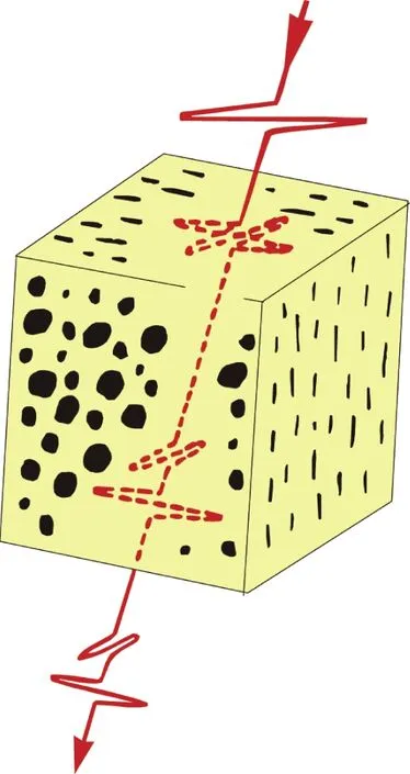
Figure 1 A schematic illustration of shear-wave splitting in the Earth’s crust containing stress-aligned cracks and fractures

1.1 Seismic anisotropy

Seismic anisotropy refers to the geophysical phenomenon by which seismic wave velocity changes with the direction of measurement in a rock or rock structure.There are two common types of seismic anisotropy in sedimentary basins.One is due to the presence of shales or shaly sediments,as well as sequences of thin layers,which give rise to transverse isotropy with a vertical axis of symmetry,often called vertical transverse isotropy (VTI).Another common type of anisotropy is horizontal transverse isotropy,or HTI,due to vertical fracturing.Figure 2 illustrates the geological origins of these types of anisotropy,where the seismic waves travel faster along the bedding planes in Figure 2a,than in any other direction.In the cases of fracturing in Figure 2b,the waves travel faster along the fracture planes than in other directions.These velocity differences demonstrate the seismic anisotropy.There are also observations of anisotropy with lower symmetry than TI (transverse isotropy),such as TTI (TI with a tilted symmetry axis),and orthorhombic symmetry (a combination of VTI and HTI),reported in the literature.

Within the context of exploration seismology,the type of anisotropy that causes shear-wave splitting is azimuthal anisotropy due to stress-aligned cracks,fractures,pores,or joints in the subsurface (Figure 1).The symmetry class may vary due to changes in the crack geometry,e.g.,HTI for a single set of vertical cracks,TTI for dipping cracks,and orthorhombic for vertical fractures in shales.Note that the fractured rock is modelled as an effectively anisotropic medium for seismic wave propagation and various theoretical modelling approaches can be find in the literature[30-31]; see Liu et al[32]for an overview of these theories.

1.2 Polarization and time delay

For near vertical propagation,the leading shear wave is polarized parallel to the fracture strike of a fractured medium when the medium possesses a single (or dominant) set of vertical,aligned fractures.Thus,the polarization of the fast split shear-wave can be used to infer the fracture strike of the medium through which it has propagated,using seismic data recorded either on the surface or in boreholes.However,the main factor affecting the use of polarization information for the target medium is the presence of anisotropic effects in the overburden,which may conceal the polarization in the target[33].

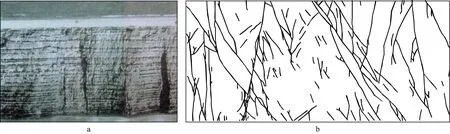
Figure 2 Two common causes of seismic anisotropy

The time delay between the fast and slow split shear waves depends on the propagation path length and direction,the symmetry of the medium,and its degree of anisotropy.Because the degree of anisotropy is mainly determined by the fracture density in each medium,time delay is a valuable attribute for the inference of fracture density from a seismic section.Time delays are usually measured by correlating the separated fast and slow shear-waves.The advantage of using the time-delay attribute lies in its simplicity:it is relatively easy to measure,and overburden anisotropy can be simply corrected for by taking the interval time delay between the top and bottom of the target.If the fracture orientation does not change with depth,layer thickness can be simply handled by normalization.

1.3 Normal reflectivity

Thomsen[34]suggested that the differential amplitudes between the fast and slow split shear-waves may be used to identify fracture zones,if these fracture zones are terminated at lithological boundaries,which has been commonly observed in outcrops.In such cases,the anisotropy caused by the fractures tends to affect the slow wave (with polarization perpendicular to the fracture strike) more than the fast wave (with polarization parallel to the fracture strike).The presence of the fractures will lower the velocity of the slow wave and cause a change in the slow wave’s impedance contrast with respect to that of the fast wave,hence a difference in reflection strength in the fast and slow sections occurs,usually causing dim spots in slow wave reflections.This phenomenon is often referred to as differential reflectivity at normal incidence.Note that anisotropy caused by macro-fracture,whose scale length is comparable with the wave length,may affect both the fast and slow split shear-waves[35].The differential reflectivity at normal incidence is a very useful indicator of fracture swarms,and thin-layer or weakly fractured reservoirs may be resolved.The main difficulty lies in maintaining and recovering true amplitude information during processing[36].

1.4 Frequency-dependent attributes

These attributes exploit the phenomenon of frequency-related changes,such as dispersion and attenuation,for predicting reservoir fluid based on empirical understandings extrapolated from laboratory measurements.Chapman[37]proposed a dynamic poroelastic theory for the frequency dependent properties of fractured rock.The model contains two scale lengths of reservoir heterogeneities:micro and meso-scale.For meso-scale fluid-filled open fractures (longer than the grain scale but still shorter than the wavelength,on the scale of a metre for typical rock properties) the theory predicts that shear-wave splitting becomes frequency dependent,with the frequency dependence being related directly to the scale lengths of the fractures,as well as to the types of fluid within the fractures.This provides a basis for relating frequency dependent seismic attributes directly to the dominant scale length of the open fractures,as demonstrated in Maultzsch et al[13],and the reservoir fluid,as shown in Qian et al[38-39].

To sum up,it is understood that shear-wave splitting is caused by stress-aligned cracks or fractures in the subsurface.The fracture strike,and probable direction of fluid flow within a fractured reservoir,can be inferred from the polarization direction of the fast split shear-wave.The time delay between the two shear-waves can give information about fracture and crack density,while differential reflectivity can help in identifying more intensely fractured zones,gas concentration,and sometimes fluid saturation.Frequency-dependent changes in time delay and reflectivity may be used to characterize fracture scale length and oil/water discrimination.Note that some complications may occur due to overburden anisotropic effects which may conceal the fracture orientation in the reservoir,and for a thin or weakly fractured reservoir,in which the time delay may be too small to determine accurately.

2 Acquisition and processing of shear-wave splitting

Due to the development of polarized sources and receivers,up to nine-component data can be recorded using different configurations of three-component sources and receivers (Figure 3a).For investigating shear-wave splitting,a configuration of two-by-two shear-wave surveys (xx,xy,yxandyycomponent (the hatched area in Figure 3a) have been used in the past[40-41],which is termed as four-component geometry.For converted shear waves,a compressional P-wave source is used and recorded with three-component (3C) receivers (the shaded area in Figure 3a).We will review the processing methods for both the four-component shear-wave and wide-azimuth converted-wave geometries,as below.

Figure 3 Data matrix for nine-component recording geometry (a).There are three orthogonal sources (x,y,and z) represented by the columns,and three orthogonal receivers (x,y,and z) by the rows.The shaded area represents the conventional three-component converted-wave geometry and the hatched area represents two-by-two shear-wave recordings (two horizonal sources and two horizontal receivers).The acquisition coordinate system (b),x,y and z,the local coordinate system,r,t,z,and the natural coordinate system,S1,S2,z.The x and y directions are also known as the inline and crossline directions,respectively.S1 and S2 represent the polarization directions of the fast and slow shear-waves,respectively.Note that for converted-wave acquisition,the source line is often orthogonal to the receiver line,forming a cross spread

2.1 Processing techniques for the four-component geometry

Figure 3b shows the coordinate systems used in multicomponent seismic surveys following Gaiser[15].The acquisition coordinate system is specified by the Cartesian coordinatesx,yandz,where x is the inline direction,y is the crossline direction,and z is the vertical direction,forming a right hand coordinate system.The source centred cylindrical system is often used as the local coordinate system,and is specified byr,tandz,where r is the radial direction away from the source,t is the transverse direction,and z is the vertical.For analysis of shear-wave splitting,the so-called natural coordinate system (S1,S2 andz) is also used,where S1 and S2 represent the polarizations of the fast and slow split shear-waves,respectively.

The four-component shear-wave survey with two horizontal sources and two horizontal receivers,as shown in the crossed area in Figure 3a,forms a data matrix,D(t):

(1)

where the left column,xx(t) andyx(t),are the inline (x-axis) traces from the inline and crossline sources,respectively,and the right column,xy(t) andyy(t),are the crossline (y-axis) traces from the inline and crossline sources,respectively.This data matrix concept is very important for processing and interpreting shear-wave splitting.

The purpose of processing multicomponent shear-wave data is to preserve and recover the three major attributes (polarization,time delay and principal reflectivity).The shear-wave data matrix represents a tensor wavefield,and conventional P-wave data processing methods are not directly applicable.The basic approach,as reported in the literature,is to separate the tensor wavefield into the principal vector wavefields containing the fast (S1) and slow (S2) shear waves only.The fast and slow shear-waves may then be processed separately by conventional scalar methods,such as statics correction,velocity analysis,normal moveout correction,etc.For short spreads and near vertical propagation,the data matrixD(t) is symmetric sincexy(t) andyx(t) are equal due to wavefield reciprocity.There are two orthogonal eigenvectors in a two-by-two symmetric matrix,and the fast and slow shear wavefields are represented by the two eigenvector components ofD(t).

Note that for isotropic media,no coherent signals would be recorded in the off-diagonal components of the data matrixD(t).Therefore,the presence of coherent and strong shear-wave signals in the off-diagonal components ofD(t) indicates shear-wave splitting due to azimuthal anisotropy.The data matrixD(t) can be diagonalized by rotating the source and receiver acquisition coordinate systems into the natural coordinate system,if the rotation angle is known.This is because the source in the fast direction only excites the fast split shear-wave which will only be recorded by the receiver in the fast direction.Similarly,the source in the slow direction only excites the slow split shear-wave which will only be recorded by the receiver in the slow direction.This can be expressed as,

(2)

To perform the rotation operation in equation (2),estimation of the rotation angleθis required.Thomsen[34]and Alford[40]proposed a rotation scanning procedure which rotates the source and receiver axes using a series of angles in order to find the angle that minimizes the energy in the off-diagonal elements (thexyandyxcomponents) of the data matrix.Li and Crampin[42-43]suggest a Linear-Transform Technique (LTT) as an alternative to the rotation scanning technique.The linear-transform technique contains four linear-transforms,which effectively recast the complicated shear-wave motions in the recording coordinate system into linear motions in the transformed coordinate system.Then the rotation angle can be determined analytically by linear regression from these linearized components.In principle,all these methods assume that the amplitudes of the two split shear-waves are eigenvalues of the data matrix.This heralded a series of analytical techniques for determining the rotation angles for shear-wave VSPs by Zeng et al[44-45].The shear-wave data examples presented in this paper have been processed using the LTT algorithms.For completeness,we include some basic equations of LTT.From equation (2),the data matrixD(t) can be expressed as:

(3)

Introducing four linear transforms as:

(4)

and applying to equation (3) with some manipulations,gives,

(5)

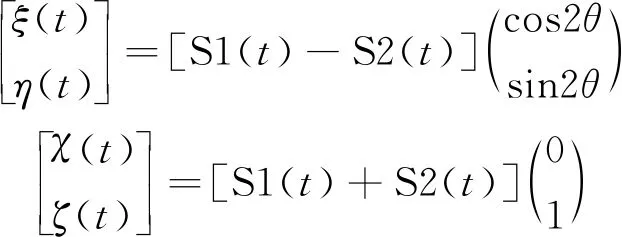
Therefore,the rotation angleθcan be determined from the transformed vector[ξ(t)η(t)]Tby linear regression as:

(6)

The summation is over a chosen time window,or the entire recorded time,andtrepresents the starting point of the chosen window.If we apply equation (6) for each time sample,instantaneously (e.g.,the length of the time window is one sample),then we obtain one angle for each sample.This is referred to as a polarization log,or instantaneous polarization trace[43].

Another major challenge in processing the split shear-waves involves near-surface and overburden amplitude corrections to recover the shear-wave information associated with the target zone.The shear-wave will inevitably be affected by acquisition errors,near-surface irregularities,and overburden anomalies.Winterstein and Meadows[46]developed a layer-stripping algorithm for the VSP context,and MacBeth et al[47],and Thomsen et al.[48]modified this stripping procedure for reflection data.Li[36]presented a more robust and practical procedure for amplitude correction in multicomponent shear-wave data; the procedure includes a pre-stack surface-consistent correction and post-stack overburden scaling.

2.2 Wide azimuth acquisition geometry for converted waves

Consider the off-line shooting cross-geometry as shown in Figure 3b for converted waves,where the source inline direction is orthogonal to the receiver inline direction.For thei-th source-receiver azimuthαimeasured clockwise from inline source direction,the horizontal componentsdir(ts) anddit(ts) in the local coordinate system (r,t) can be written as,for shear-waves only,following Li[16]:

(7)

wheretsis the shear-wave travel time after P-to-S conversion,Δ =θ-αiis the angle between the fracture strike and thei-th source-receiver azimuth,λ1andλ2are propagating functions for the fast and slow wave,respectively,and PSiis the effective shear-wave source for thei-th source-receiver azimuth due to conversion.Note that based on Huygens’ principle,the wavefront upon conversion can be treated as an effective source which excites the subsequent up-going shear wave.The magnitude of this effective shear-wave source is related to the raypath of the first P-wave leg and the P-to-S conversion coefficient at the interface.For simplicity,it is assumed that the effects of PSican be compensated for during processing.It follows from Equation (7) that:

(8)

dit(ts,-Δ)=-dit(ts,Δ)

(9)

This implies that if the source-receiver azimuth is parallel or perpendicular to the fracture strike,the energy in the transverse component vanishes,and that the wave forms show a polarity reversal every 90 degrees.Here,full-wave modelling using the reflectivity method[49]is carried out to illustrate this feature.Table 1 shows the model parameters,and Figure 4 shows the modelling results.Travel time variations are observed on the radial component (Figure 4a),and polarity reversals on the transverse component (Figure 4b).Li[16]is the first to recognize the importance of the polarity reversal in the transverse component for analysing shear-wave splitting.His theoretical prediction was later con-firmed by real data[50],and subsequently evolved into a standard procedure for analysing shear-wave splitting in converted-wave data[27,51].Note that Garotta and Granger[52]analyse the amplitude ratios of the transverse and radial components utilizing the amplitude dimming effects in equation (8).

Table 1 Elastic parameters for the synthetic model in Figure 4

Figure 4 Azimuthal gathers of radial (a) and transverse (b) components calculated for the three-layer model in Table 1 where the second layer is fractured chalk and the fracture strike is 60 degrees from the source line direction.Note the azimuthal variation in travel time at the radial component, the polarity reversal in the transverse component that happens every 90 degree, and that the angles at the zero crossing traces represent the fracture strike or the fracture normal

Consider the source-receiver azimuth that is orthogonal to thei-th azimuth,and denote this as thej-th azimuth.From equation (7),the horizontal components of thej-th azimuth may be written as,

(10)

Following Li[16],after correcting the ray-path difference by moveout correction,and compensating the effects of the effective sources by amplitude scaling,the recorded horizontal components in these two orthogonal azimuths can be combined to form a two-by-two data matrix,

(11)

This has the same form as the data matrix in Equation (3).Therefore,Alford rotation or the LTT as discussed in the previous section can be applied as well.The polarization azimuth can be solved by minimizing the off-diagonal elements of the data matrixDij(ts,Δ).This method was first proposed by Gaiser[14]for analysing converted wave splitting in 3D land acquisition,and was subsequently reformulated for marine sea-floor data by Li[16]and Dellinger et al[53].As interest in land converted waves continued to increase,Bale et al.[54],Haacke et al.[55]and Simmons[56]developed more formal inversion algorithms for the fast polarization azimuth and time delay of the split shear-waves.

Compared with the polarity reversal in equation (9),the data matrix approach in equation (11) requires proper correction of the moveout and proper scaling of the off-diagonal components to compensate for the differences in the conversion coefficients.Thus,this procedure may be best suited for post-stack analysis,since forming a two-by-two data matrix by orthogonal azimuths may only be valid for near-vertical propagation.Also note that during acquisition,the horizontal geophones are actually orientated in the inline and crossline directions of the acquisition coordinate system (x,y),and additional rotation from the acquisition coordinate system (x,y) to the local coordinate system (r,t) is required.

3 Observations of shear-wave splitting

In the 1980’s,Amoco Production Company acquired four-component (xx-,xy-,yx- andyy-components) and five-component (xx-,xy-,yx- andyy- plus thezz-components) surveys[7].The purpose of these surveys was to investigate whether shear-wave splitting could be used for fractured reservoir characterization,utilizing particularly the dim spots in slow shear-wave sections.This is useful when the fracture porosity is too low to significantly alter the P-wave impedance contrast.This approach has been successfully applied to locating fracture swarms in the Austin Chalk in Texas[41,57]using 2-D lines,and guiding horizontal drilling into productive zones.The approach has also been employed in large 3-D surveys[58],and for a variety of reservoirs with fractured dolomites,sandstones,and coals.In the latter,the high/low impedance contrast now produces a brightening of the slow shear-wave horizon[59].Despite these successes,these two-by-two shear-wave source surveys are not shot on a routine basis due to the expense in setup and data quality issues.

In the 1990’s,whilst shear-wave studies continued in consortium projects,such as the Reservoir Characterization Project (RCP) at the Colorado School of Mines,and the Edinburgh Anisotropy Project (EAP) at the British Geological Survey,much emphasis was put into the acquisition of shear-wave VSPs[12].This decade also marked a rapid development in converted-wave seismic exploration.Garotta and Granger[52]first reported the acquisition and processing of 3D3C data.This interest in converted waves was then rekindled in the mid 1990’s due to the success in using P-to-S converted-waves to image beneath gas clouds in the Tommeliten field in the North Sea[60-61].It was then followed by surveys in the Valhall[62-63]and Alba[64]fields in the North Sea,as well as various onshore converted-wave surveys thereafter[65-66].

In the past twenty years since 2000,with the advent of the MEMS (micro-electronic-mechanic-system) sensor,the acquisition cost of converted wave data has substantially reduced,and converted-wave surveys in land seismic acquisition have become commercially viable.Converted-wave surveys are often shot in a wide azimuthal fashion,utilizing the azimuthal variations in seismic attributes[50,67-68].As interest in unconventional reservoirs grows in the industry,a rapid development of converted-wave applications in shale gas exploration has taken place in the last ten years[69-70].

In China,initial shear-wave exploration was carried out in the late 1980’s and early 1990’s[71].Experimental studies continued throughout the 1990’s and early 2000’s[72-73].In particular,the last fifteen years have witnessed the rapid development of converted wave exploration in China[74-75].One of the most successful commercial applications of 3D3C converted-wave exploration was from Xinchang gas field,Sichuan[76-78].This is followed by a series of surveys across China including Changqing in the west[79],Shengli in the east[80],Daqing in the north[81-82],Tarim Basin[83]in the northwest,and Sanhu[84]in the west,to name but a few.Nowadays,3D3C surveys are almost routinely acquired in Sichuan Basin in the southwest of China[85-87].We will select a few representative examples to illustrate this historical process covering shear-wave reflections and VSPs in north America and converted-wave surveys in China.

3.1 Shear-wave splitting in reflection surveys

Willis et al[7]presented four-component shear-wave data across fourteen sites in the west of North America,and except for two sites,shear-wave splitting was observed in all other sites with the degree of splitting averaging about 1%～2%.Despite the small percentage,the accumulated time delays reached 60ms at 4s depth.These shear-wave surveys were repeated along the Austin Chalk formation in Texas and the degree of splitting in these data was up to 3% on average.In 1988,the shear-wave data acquired along the Austin Chalk were donated to the Edinburgh Anisotropy Project for reprocessing and interpretation,and the results were published in Li et al.[41,88-89].Figure 5 shows a typical data matrix acquired in Texas,and its corresponding stacked sections for the fast and slow shear-waves,which represented the best data quality at the time.Strong coherent shar-wave energy was observed in the off-diagonal components,indicating shear-wave splitting (Figure 5a),and there is a consistent time delay between the fast and slow sections (Figure 5b).However most of the delay was in the overburden,and the interval delay for the Austin Chalk is small and averaged 6～8ms,only 1-2 samples,whilst the cumulative delay is up to 30～40ms.The polarization azimuth of the fast waves representing the dominant fracture orientation is constant in the subsurface and varied from N40oE to North100oE along the chalk from southwest to northeast.A constant fracture azimuth with depth and a relatively thick chalk provided a favourable geological setting for the application of shear-wave splitting.These observations in the Austin Chalk were largely consistent with other studies in North America[58-59,90],and confirmed by VSPs as shown in Figure 6 below.

3.2 Shear-wave splitting in VSPs

Shear-wave VSPs provide a more direct and ac-curate measurement of shear-wave splitting at depth.Figure 6 show four-component shear-wave VSPs at Devine,Texas.Here the Austin Chalk locates at about 800m at depth.The VSP data in Figure 6a are of much higher frequency band and S/N ratio than the surface data in Figure 5a.Figure 6b shows the corresponding fast azimuth and time delay.The polarization azimuth is constant with depth and at the angle N50°E which is consistent with the structural trend.Most of the time delays are in the overburden,and the interval time delay for Austin Chalk is very small and about 2ms.

Figure 5 Observation of shear-wave splitting in reflection seismic data in the Austin Chalk,Texas

These observations of shear-wave splitting were broadly in agreement with Winterstein et al.[12]who documented measurements of shear-wave splitting in 23 VSPs from west America.They found that the largest amount of shear-wave splitting (4% or above) is confined in the near surface at less than 1200m at depth,and the splitting in the reservoir is often smaller than the overburden.Furthermore,the polarization azimuth,as well as the magnitude of splitting,was often found to be very consistent with depth interval over hundreds of meters.These findings have very significant implications for shear-wave reflection data:①layer-stripping methods may not be necessary for shear-wave reflection data,and ②very high quality data may be needed to quantify shear-wave splitting over the reservoir interval.

3.3 Observation in converted-wave surveys

For wide-azimuth converted-wave surveys,the most diagnostic feature of shear-wave splitting is the polarity reversal in azimuthal gathers of the transverse component,as shown in the modelling results of Figure 4.Figure 7 shows a real data example from the Sanhu gas field,China.When the time-delay is more than half cycle of the wavelet,as in this case,the travel time variations in the radial component alternate between the fast and slow wave.Thus the time-delay can be directly measured from the radial component at about 50ms at a depth of 1.2s,giving rise to about 4% converted-wave splitting,which is very significant (Figure 7a).The polarity reversal is observed at 65 degrees and repeated every 90 degrees (Figure 7b).

Figure 6 Observation of shear-wave splitting in VSPs from Devine,Texas

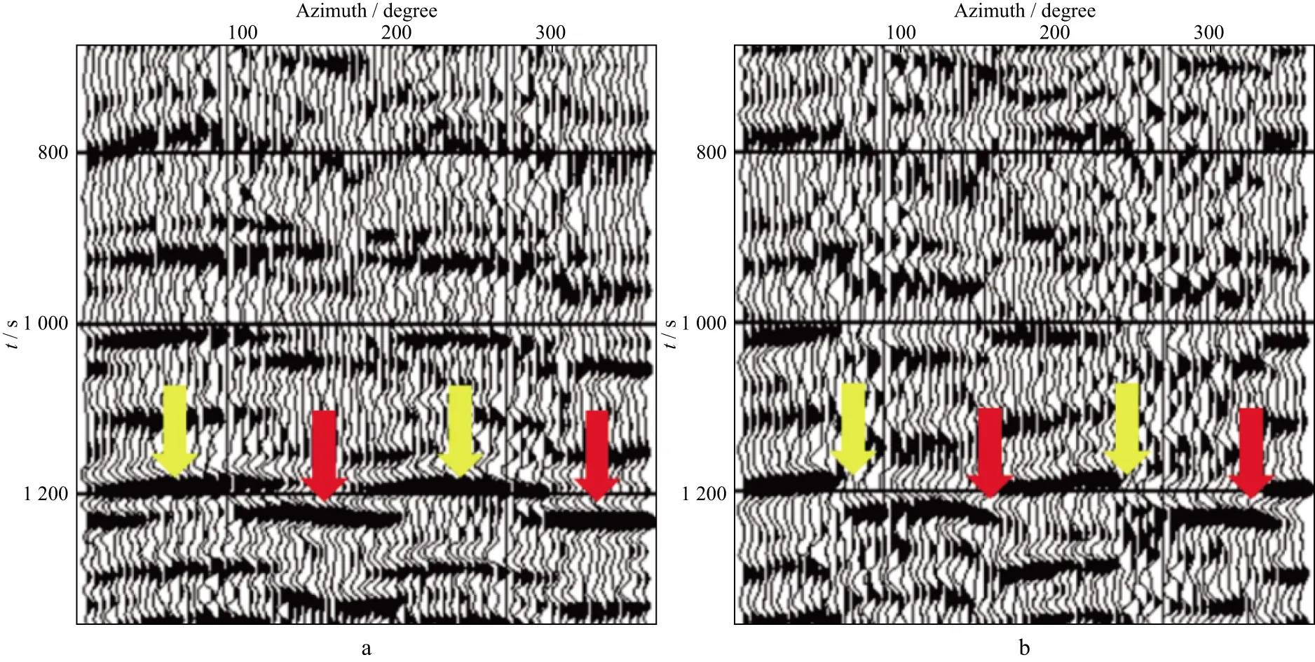
Figure 7 Observation of shear-wave splitting in PS converted-waves,showing the azimuthal gathers of (a) the radial and (b) transverse components,where the radial displays travel time variations and the transverse component shows polarity reversal every 90 degrees.Yellow arrows indicate the fast azimuth,and red arrows indicate the slow azimuth.Data from the Sanhu gas field,Qinghai,China

Another example of azimuthal travel time variation and polarity reversal is shown in Figure 8 from the Xinchang gas field in west Sichuan,China.When the delay is less than half cycle of the wavelet,sinusoidal variations of travel times can be observed in the radial component (Figure 8a),whilst polarity reversal remains the same in the transverse component (Figure 8b).

Figure 8 Azimuth-sorted CIP gathers of (a) radial and (b) transverse components from Xinchang gas field,Sichuan,China[91]

4 Applications of shear-wave splitting

The common application of shear-wave splitting is the use of shear-wave attributes,such as polarization,time delays and differential reflectivity,to map fractured reservoirs.Over the years,applications of shear-wave splitting have been extended to detect fracture scale-length and reservoir fluid type[13,38].Furthermore,temporal changes of shear-wave splitting in multicomponent time-lapse (4-D) seismic offers great potential in monitoring reservoir changes during production for improving recovery efficiency and finding by-passed oil[92].Here,we select four examples in the literature to illustrate the application of shear-wave splitting.

4.1 Example 1:Austin Chalk

Due to limitations in shear-wave data quality,in early applications the focus was to use the dim spots in the slow shear sections to delineate fractured reservoirs,such as in the Austin Chalk,Texas.The area is relatively flat and the fracture orientation remains constant with depth (Figure 6),which made it a good place to test shear-wave technology.Figure 9 shows an example from the Giddings field to illustrate the correlation of dim spots to the fracture cluster encountered by horizontal drilling.The survey line in Figure 9a had a horizontal well drilled on it with supporting mud logs for identifying fracture zones.W4 marks the horizontal well with mud logs taken to verify the fractures.Figure 9b shows a portion of the slow S2 section,which highlights the amplitude anomaly and its intercept with the horizontal well.The fractures and the amplitude anomalies are all projected onto the surface and are shown in Figure 9a.There is clearly a very good correlation between the dim spots in the slow wave section and the fracture swarms identified by the mud logs.Inaddition,the overall shear-wave anisotropy represented by the time delay was also found to correlate well with local production[57,88].Similar applications were repeated elsewhere[58-59].

Figure 9 Location map(a).The light dashed line represents the survey line,and the small black boxes on the survey line represent the dim spots interpreted from the slow (S2) section below.The solid line trending to the northwest represents the horizontal borehole,and the open square boxes on the borehole are fracture swarms determined from mud logs.The outline square box represents the lease boundary.The solid dots are the surface locations for the producing wells drilled to the Austin Chalk.A portion of the S2 seismic section(b) showing amplitude dim spots,with heavy vertical bars marking the lease boundary; the reversed L-shaped line marks the borehole.The seismic section has the same lateral scale as the map in (a)[89]

4.2 Example 2:Fractured tight sandstone reservoir

A good example of using converted wave data for characterizing fractured reservoirs comes from the Xinchang gas field in Sichuan,China,where the reservoir formation is a tight sandstone,buried at around 5,000 meters depth from the surface.Due to the very low porosity and matrix permeability,production is entirely dependent on fractures.In 2005,a 3D3C multicomponent survey was acquired to characterize the fracture reservoirs,and the main attributes used are the polarization and time delay of split shear-waves.Compared with the early shear-wave example in Figures 5 and 9,the data quality in Xinchang (Figure 8) was substantially improved allowing accurate measurements of the polarization and time delays of the reservoir formation.The results are shown in Figures 10,where the colour displays the time-delay between the fast and slow shear-waves,and the short line represent the direction of fast wave polarization.W851 is a highly productive well,which is characterized by a higher amount of shear-wave splitting.The roman numerals mark the reservoir quality.Type Ⅲ targets are of the highest quality.

4.3 Example 3:Characterizing gas deposits

The example is from Sanhu,Qinghai in west China.There are wide distributions of gas deposits in the shallow unconsolidated sediments of the Sanhu area.A 3D3C dataset of 60km2was acquired,and significant converted shear-wave splitting is observed,as shown in Figure 7.The final migrated fast and slow shear-wave sections are shown in Figure 11.Based on the theoretical modelling of Qian et al.[38],the presence of gas affects the slow shear-wave more than the fast wave,and bright spots are expected at the slow shear-wave section as gas accumulates.This prediction was observed in the Sanhu converted-wave data.As shown in Figure 11,at the K9 horizon,the slow shear-wave shows clearly a bright response at the Well location.Therefore,a differential attribute between the fast (AS1) and slow (AS2) amplitudes,AS1-AS2,is created to delineate the gas deposits,as shown in Figure 12.The negative bright amplitudes highlighted the gas pockets,which agreed with the drilling results as indicated by the producing wells.This opens a new application of shear-wave splitting.

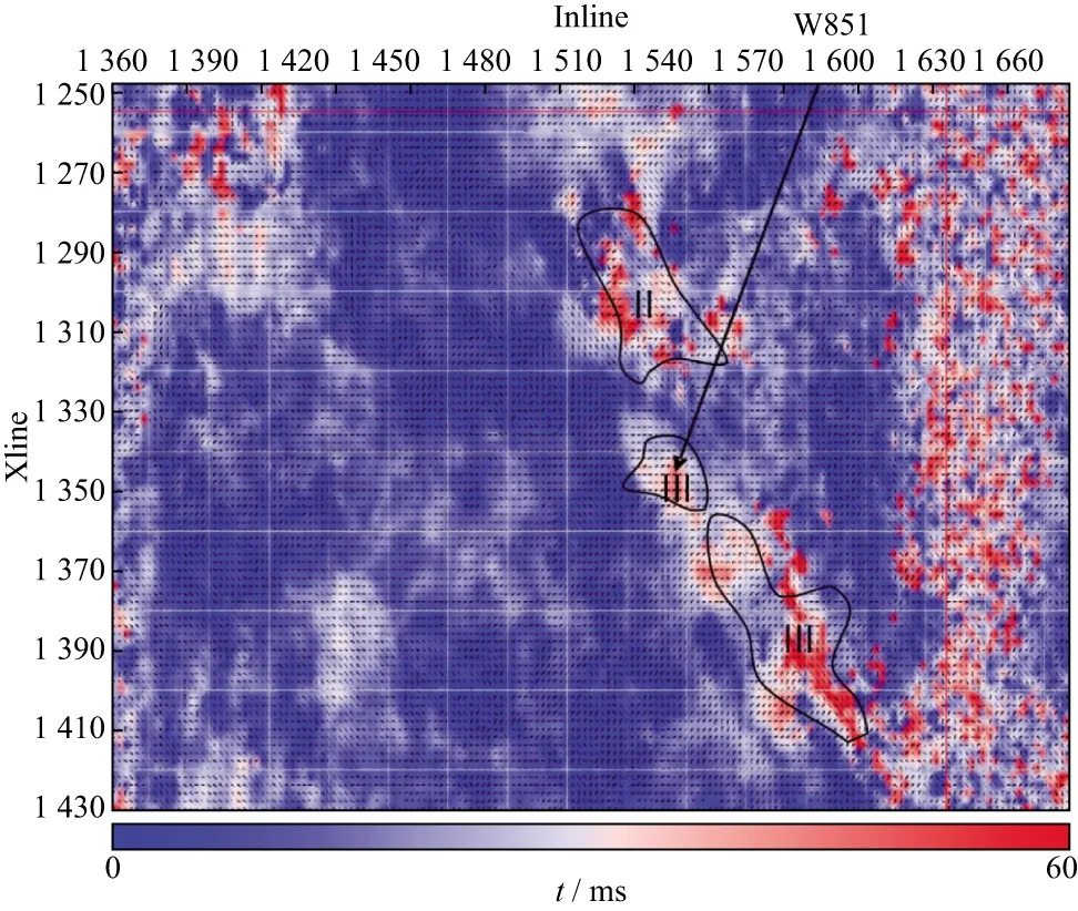
Figure 10 Polarizations and time-delays of the fast and slow shear-waves for the target horizon in Figure 8.The bars show the polarization and colour contour shows the time delay.The Roman numerals indicate reservoir quality[91]

4.4 Example 4:oil/water discrimination

As we know,oil and water have similar impedance values,and therefore it is difficult to distinguish them by inverted impedance from seismic data.However,oil and water have significant differ-ences in viscosity and it could be useful if the effects of viscosity can be detected from seismic waves.Chapman and colleagues[37,93]proposed a multiscale fractured model accounting for the effects of fluid mobility which is defined as the ratio of permeability to viscosity.According to Chapman et al[93],the magnitude of shear-wave splitting as a function of frequency varies with fluids of different viscosity as shown in Figure 13a.This prediction was later confirmed by laboratory measurements from fractured synthetic sandstones[94],as shown in Figure 13b.Qian et al.[38]and Luo et al.[39]attempted to apply these findings to real data acquired in Shengli oilfield in 2005,and the results are shown in Figure 14.An oil-and a water-producing well were selected that intersect the seismic data,and the time delays increase more sharply through the water formation (Figure 14b) than through the oil formation (Figure 14a),leaving a bright spot in the time-delay gradient section (Figure 14c).This confirms the theoretical prediction as well as the laboratory observation.However,careful calibration and modelling,and sufficient data quality,are required for a successful application.

Figure 11 The migrated (a) fast and (b) slow shear-wave sections from Sanhua that intersect a gas producing well T9; note the amplitude brightening at the slow section where T9 penetrates horizon K9

Figure 12 Differential fast (S1) and slow (S2) shear-wave amplitudes (AS1-AS2) of the target layer K9 from the Sanhu 3D3C data in Figure 11,showing an area of 18km2 of gas concentration,in agreement with drilling results

Note that the fracture scale length also affects the fluid mobility,hence the magnitude of shear-wave splitting which results in the magnitude of splitting varies with frequency as the fracture length varies.Maultzsch et al.[13]observed this phenomenon in a four-component VSP and successfully inverted these changes to characterize the fracture scale length.

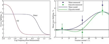
Figure 13 Predicted values of shear-wave splitting (a) as a function of frequency for oil and water saturations [38];laboratory measurements of shear-wave splitting (b) from synthetic rocks.Dots are measured and solid lines are calculated;green for Glycerin,black for water.After Tillotson et al[94]

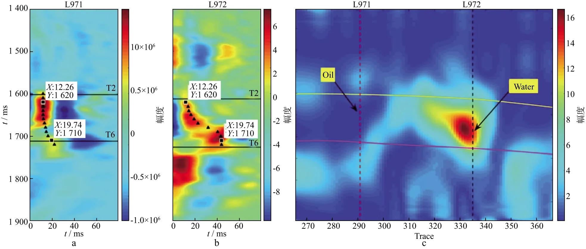
Figure 14 Time-delay spectrum of the fast and slow shear wave traces near the oil well (a) L971,(b) the water well L972,and (c) their corresponding gradient section calculated by the time-delay values at (a) and (b).T2 and T6 correspond to the top and bottom interface of the target interval; the red and black dotted lines represent the locations of oil and water wells.Modified from Luo et al[39]

5 Discussions and conclusions

This paper has discussed the concept of shear-wave splitting and its historical development for characterizing fractured hydrocarbon reservoirs.In the past forty years,the exploration industry has developed specific polarized sources and receivers,specific four-component shear-wave and wide-azimuth converted-wave geometries for recording shear-wave splitting in multicomponent VSPs and reflection surveys.Hydrocarbon reservoirs containing aligned fractures are anisotropic and cause shear-wave splitting,and examination of the resultant split shear-waves can give us vital information about reservoir structure.Hydrocarbon reservoirs become increasingly complex,and examining the resulting frequency-dependent information in shear-wave splitting can provide vital information about fracture scale length and fluid properties.The examples reviewed here are of particular importance,as they demonstrate not only proven applications,but also the undoubted potential of shear-wave splitting in reservoir characterization.

Due to these efforts,it is now understood that shear-wave splitting occurs widely in sedimentary basins with an average degree of splitting of about 1～3%.However,it was also revealed that most of the splitting was associated with the near surface (<1200m),and current successful examples are all restricted to some favourable near-surface and reservoir conditions,such as simple near-surfaces and relatively thick reservoirs that can be resolved by the seismic wavelet.Also there is often only one single set of dominant fractures in the subsurface and its orientation remains the same at depth.Although these conditions seem to be very restrictive,they are,in fact,quite common in sedimentary basins which have not been subjected to heavy tectonic movement through their geological history.

There are still two main challenges facing us on the road to realizing the full potential of shear-wave splitting,as well as the routine application of multicomponent seismic surveys.First,accounting for the effects of the near surface is still a challenge.Shear-wave velocities vary sharply in the near surface,and degrade the data quality.The near surface also tends to be heavily anisotropic.A full and comprehensive near surface survey may have to be considered.Another option is to bury the receivers in the ground,although both of these measures will increase the cost of acquisition.

Secondly,accounting for the characteristics of shear-wave or converted-wave propagation is still difficult.Due to overburden velocity and anisotropic variations,as well as imperfect velocity models in imaging,it is a challenge to reconcile images of different wave types and quantify the splitting effects associated with the reservoir interval,particularly in the absence of sufficient fold coverage,frequency bandwidth and S/N ratio.Therefore,one must acquire shear-wave or converted-wave data with sufficient fold,and uniform sampling across all offsets and azimuths.Again,this will increase the cost of acquisition.

In conclusion,the discovery of shear-wave splitting and its potential applications to characterizing fractured reservoirs is a major milestone in the development of exploration seismology.However,shear-wave or converted-wave data quality and the cost-effectiveness of shear-wave or converted-wave data acquisition are the main hurdles.Only when they become comparable with that of the P-wave,can the full potential of shear-wave splitting be realized.Recent success in the Sanhu gas field in China heralds a major breakthrough in this direction.

Acknowledgements:We thank BGP and CNPC for permission to show the Sanhu data,and SinoPec for showing the Xinchang data.We thank David Booth for his comments,and we thank the sponsors of the Edinburgh Anisotropy Project (EAP) of the British Geological Survey (BGS).