-, -

(School of Mathematics, Sichuan University, Chengdu 610064, China)

Abstract: This paper introduces and analyzes a full augmented mixed finite element method for the nonlinear elasticity problems with strongly imposed symmetry stress tensor. The mixed method includes the strain tensor as an auxiliary unknown, which combines with the usual stress-displacement approach adopted in linear elasticity. By introducing different stability terms, we obtain an augmented mixed finite element variation formulation and a full augmented mixed finite element variation formulation. In order to obtain the well-posed of the two schemes, we adopt different finite element spaces to approximate the unknowns and derive the optimal error estimate. Finally, a numerical example is presented to confirm the theoretical analysis.

Keywords: Nonlinear elasticity problem; Two-fold saddle point formulation; Augmented-mixed finite element method

1 Introduction

Stable mixed finite elements for linear elasticity, such as PEERS of order 0, also leads to well-posed Galerkin schemes for the nonlinear problem. In Ref.[1], the authors extend the result from Ref.[2] and show that the well-posedness of a partially augmented Galerkin scheme is ensured by any finite element subspace for the strain tensor together with the PEERS space of orderk>0 for the remaining unknowns. However, the stress tentor in the two papers is asymmetrical, which leads to introduce a further unknown named rotation. So they both have four variables, that is, the strain tensor and the usual stress-displacement-rotation.

In this paper, we attempt to deal with strongly imposed symmetry strain in the nonlinear elasticity problem, which makes the unknowns less than that of Refs.[2] and [3] and lets the expression of equations much briefer. Moreover, we employ thek-1 degree piecewise polynomial finite element space to approximate the strain tensortand thekdegree piecewise polynomial finite element space to approximate the stress tensorσand the displacementu. An advantage of this method is that these elements can keep theSspace same accuracy withR-Tspaces of orderkfor the stress tensor while substantially decrease the number of degrees of freedom under the same convergence degree. Finally, we apply classical results on nonlinear functional analysis to prove the well-posedness of the resulting continuous and utilize the usualCe′aestimate to derive the optimal order error estimation.

2 Problem statement

to denote the transpose, the trace, the deviator of a tensorτand the tonsorial product betweenτandξ. Then, we useHm(Ω)to denote the Hilbert spaces on Ω, ‖·‖mto be its norms. Whenm=0, we writeL2(Ω),‖·‖0instead ofHm(Ω) and ‖·‖m. We introduce the divergence spaces:

The Hilbert norms ofH(div;Ω), andH(div; Ω;S) are denoted by ‖·‖divand ‖·‖H(div;Ω;S).

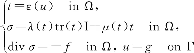
divσ=-fin Ω,u=gon Γ

(1)

Then, we set

for allr∈L2(Ω) and introduce the new unknownt=ε(u)∈L2(Ω). Problem (1) adopts the equivalent form

(2)

Next, by integrating by parts, we consider the following problem:

Find (t,σ,u)∈L2(Ω)×H(div;Ω;S)×H1(Ω), such that

for all (s,τ,v)∈L2(Ω)×H(div;Ω;S)×H1(Ω).

(4)

In this section we adopt the following three steps to derive a full augmented formulation and a discrete scheme.

In the first step, we introduce the constitutive law relatingσandτmultiplied by the stabilization parametersκ0,κ1,κ2,κ3>0, to be chosen later, and add

to the first equation of (3).

In the second step, we subtract the second equation from the first equation of (3).

In the third step, we add the third equation of (3) to the first equation again.

In this way, we arrive at the following fully augmented variational formulation:

[A(t,σ,u),(s,t,v)]=[F,(s,τ,v)]

(5)

for all (s,t,v)∈X, where the nonlinear operatorA:X→X′ and the functionalF∈X′ is defined by

[B1(s),σ]-[B1(t),τ]+

(6)

Our next goal is to show the unique solvability of the variational formulation (5). We first recall the following theorem.

Then, givenF∈X′, there exists a uniquex∈Xsuch that [A(x),y]=[F,y],x∈X. Further more, the following estimate holds

In order to apply Theorem 3.1 to the fully augmented formulation (5), we need to prove first the required properties for our nonlinear operator. We begin with the Lipschitz-continuity.

‖A(t,σ,u)-A(s,τ,v)‖X′≤

for all (t,σ,u),(s,τ,v)∈X.

In turn, the strong monotonicity of A makes use of a slight extension of the second Korn inequality, which establishes the existence of a constantc1>0 such that

∀v∈H1(Ω)

(7)

The proof of (7) follows from a direct application of the Peetre-Tartar Lemma[5].

[A(t,σ,u)-A(s,τ,v),(t,σ,u)-(s,τ,v)]≥

for all (t,σ,u),(s,τ,v)∈X.

ProofGiven (t,σ,u),(s,τ,v)∈X, we observe, according to the definition ofAand the fact that the terms involvingBcancell out, that

A(t,σ,u)-A(s,τ,v),(t,σ,u)-(s,τ,v)]=

[A(t,σ)-A(s,τ),(t,σ)-(s,τ)]+

A(t,σ,u)-A(s,τ,v),(t,σ,u)-(s,τ,v)]≥

By using the the Korn inequality (7)

A(t,σ,u)-A(s,τ,v),(t,σ,u)-(s,τ,v)]≥

The well-posedness of the fully augmented formulation (5) can be established from Ref.[2].

ProofBy Lemmas 3.2 and Lemma 3.3, the proof is a direct application of Theorem 3.1.

Find (th,σh,uh)∈Xh, such that

[A(th,σh,uh),(s,τ,v)]=[F,(s,τ,v)]

(8)

for all(s,τ,v)∈Xh.

The following theorem establishe the well-posedness and convergence properties.

Theorem3.5Assume that the parametersκ0,κ1,κ2, andκ3are chosen as in Lemma 3.2. LetX1,h,M1,handMhbe arbitrary finite dimensional subspaces ofL2(Ω),H(div;Ω;S), andH1(Ω), respectively. Then there exists a unique (th,σh,uh)∈Xh, solution of (8). Moreover, there existC1,C2>0, independent ofh, such that

‖(th,σh,uh)‖X≤C1{‖f‖0,Ω+‖g‖1/2,Γ}

(9)

‖(t,σ,u)-(th,σh,uh)‖X≤

(10)

In order to develop the rate of convergence of the Galerkin solution provided by Theorem 3.5, we need the approximation properties of the finite element subspace involved. Therefore, we define

(11)

Pk+1(T) ∀T∈Th}

(12)

∀T∈Th}

(13)

The following theorem provides the corresponding rate of convergence.

Theorem3.6Assume that the parametersκ0，κ1，κ2, andκ3are chosen as in Lemma 3.2. Given an integerk≥0, letX1,h,M1,handMhbe the finite element subspatces defined by (11) ～(13), (t,σ,u)∈Xand (th,σh,uh)∈Xhbe the unique solutions of the continuous and discrete formulations (5) and (8), respectively. Suppose thatt∈Hδ(Ω),σ∈Hδ(Ω), andu∈Hδ(Ω) for someδ∈(0,κ+1]. Then there existsC>0, independent ofh, such that

‖(t,σ,u)-(th,σh,uh)‖X≤

Chδ{‖t‖δ,Ω+‖σ‖δ,Ω+‖u‖δ,Ω}.

ProofIt follows from theCe′aestimate (10) in Ref.[3].

4 Numerical example

In this section we present a numerical example illustrating the performance of the Galerkin schemes (8). We considerk=0. LetNstand for the total number of degrees of freedom (unknowns),handh′ denote two consecutive meshsizes with corresponding errorεandε′. The total errors are given by

ε(t)=‖t-th‖0,Ω,ε(σ)=‖σ-σh‖0,Ω,

ε0(u)=‖u-uh‖0,Ω,

In addition, we introduce the experimental rates of convergence

In the example, we set Ω=]0,1[×]0,1[ and choose the datafandg, so that the exact solution is given by

for all (x1,x2)t∈Ω.

In Tab.1, we summarize the convergence history of the example. We observe that theO(h) predicted by Theorems 3.5 (withδ=1) is obtained by all the unknowns.

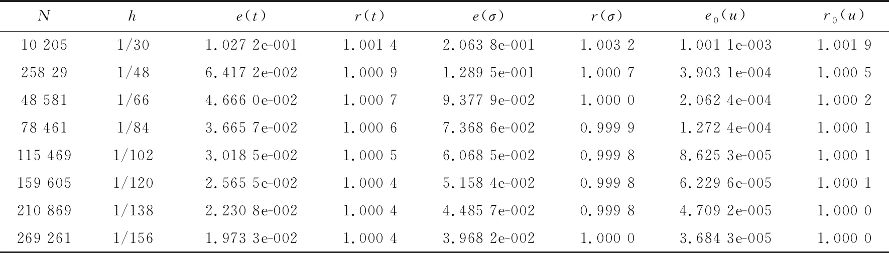
Tab.1 The convergence of the unknowns in the fully-augmented formalation