Chun-Feng Zhang(章春锋), Wei Wang(汪伟), Si-Guang An(安斯光), and Nan-Ying Shentu(申屠南瑛)

Department of Mechanical and Electrical Engineering,China Jiliang University,Hangzhou 310016,China

Keywords: mesh generation,smoothing function,finite element,electromagnetic calculation

1. Introduction

With its favorable ability to adapt the geometric shape of the field boundary and the variation of the physical properties of the medium,the finite element method has become one of the powerful numerical calculation methods for numerical analysis and optimal design of electromagnetic field.[1,2]Generally speaking,the finite element analysis is divided into three stages: modeling, calculation and solution, result processing and evaluation. Their proportions of time spent in each stage are 40%–60%, 5%–10%, 30%–50%, respectively. For complex geometry and fine meshes,it may take too long to generate a qualified mesh. The mesh generation time may account for more than 90% of the total CPU time in the whole numerical simulation process.[3–5]Therefore,how to effectively improve the speed and quality of mesh generation is crucial to the finite element method.

To improve the efficiency and quality of finite element meshing, endeavors have been made mainly in parallel mesh generation, mesh smoothing methods and mesh optimization process. Parallel mesh generation techniques can be classified as discrete domain decomposition (DDD) parallel meshing and continuous domain decomposition (CDD)parallel meshing.[6–9]The DDD parallel meshing generates coarse meshes sequentially for the input boundaries firstly and uses the mesh or graphics division technique to refine the coarse mesh. In the CDD method, more methods such as quadtree/octree,spatial sorting can be used to decompose the domain. Parallel mesh generation can increase the speed to mesh the solving domain based on decomposition. However,most parallel mesh generation methods need lots of memory to generate large-scale meshes;data dependence,load balancing,and the robustness of the method are still needed considering.

Currently, there are three main approaches for mesh smoothing: Laplacian and Winslow, optimization-based method, and physics-based method.[10]In the Laplacian and Winslow method, nodal positions are updated by the arithmetic mean of connected nodes and minimizing specific mesh quality metrics, respectively, to prevent mesh from folding.[11–13]In the optimization-based smoothing method,the nodal positions can be derived by solving local or global optimization problems with different types of objective functions.[14]In the physics-based method, the mesh is considered as physics system to improve the shape of the element.[15,16]The mesh smoothing method can improve both the average quality of the mesh and the efficiency the mesh generation. However,iterations are often involved in the mesh smoothing which is time-consuming. A fast mesh smoothing method is a persisting pursuit for the mesh generation algorithm.

Techniques and schemes are also proposed in the mesh optimization process to promote the performance of the mesh generation. A mesh quality metric alternation scheme is used in the mesh optimization process to obtain the high-quality mesh.[17,18]Some literature proposes a novel automated highorder unstructured triangular mesh generation method for the two-dimensional domain.[19,20]A mesh-generation framework for image representation based on data-dependent triangulation was proposed.[21]These methods have improved the performance of mesh generation to some extent.

In order to improve the convergence speed of mesh iteration and ensure the quality of mesh generation in finite element analysis to a forward step, several improvements are made based on the Persson’s algorithm. An image boundary extraction algorithm based on path optimization is introduced to avoid the interaction between the computer-aided design (CAD) and the finite element analysis software, which provides an alternative method to build the geometric boundary for the solving domain. Based on Persson’s algorithm,identification algorithm for the location of nodes in polygon area is proposed to determine the state of the boundary node.Finally,a novel force-based mesh smoothing algorithm is proposed to improve the mesh quality and convergence speed of the mesh generation method.

2. Persson’s algorithm

In the Persson’s algorithm, the signed distance functions is used to specify and describe the geometric regions to be meshed.[15]The signed distance functions specify the shortest distance from any point in the space to the boundary of the domain,where the sign of the function is positive outside the region, negative inside, and zero on the boundary. This definition is used to identify whether the point is inside or outside the geometric domain. The geometric field Ω can be implicitly defined as

The Persson’s algorithm is based on the analogy between triangular meshes and two-dimensional truss structures. The edges of the triangle correspond to the bars, and the vertexes correspond to the nodes of the truss. Each of the bars in the truss structure has a force function f(l, l0).

Persson’s algorithm determines that the relationship depends on length l and unextended length l0. At every boundary node,there is a reaction force acting normally on the boundary. This force is just large enough to prevent the node from moving outward. α is usually set to be 1,it is reasonable to require f =0 for l=l0. The positions of the joints are found by solving for a static force equilibrium in the structure.

The equilibrium problem corresponds to a nonlinear equation: F(p)=0,where F(p)is an N-by-2 array in which the first column contains x-components of the forces,and the second column contains the y-components of the forces. A simple way to solve the equation is to introduce an artificial time-dependent solution. For some p(0)=p0,the ODES system in non-physical units is considered as follows:

If a constant solution is found,the system F(p)=0 is satisfied.The system uses forward Euler method for approximation. In the case of discrete time tk=kΔt, the approximate solution pk≈p(tk)is updated as follows:

Persson’s algorithm is simple and compatible. For some regions with geometric and mathematical background, it is relatively easy to create signed distance functions; however,for other regions, distance functions cannot be expressed quickly and accurately, and some are even difficult to express. For mesh smoothing, Persson’s algorithm tries to optimize the node locations by a force-based smoothing procedure. This method usually generates high-quality mesh elements,but sometimes extremely low-quality elements are obtained, which will seriously affect the accuracy of the finite element calculation;and due to the fact that the force balancing method used in this algorithm has only a repulsive force,it is inevitable that frequent iterations will occur, which may lead low efficient mesh to be generated.

3. The proposed algorithm

Due to the lack of Persson’s algorithm in the definition of complex polygons, and room for improvement in the efficiency and quality of mesh generation, some improvements are developed to speed up the convergence and also guarantee the quality of the output mesh.

3.1. Image boundary extraction algorithm based on path optimization

The solving domain of finite element analysis is built generally by the CAD or the modeling operation in finite element analysis software. Modern CAD systems tend to integrate finite element analysis tools into the design environment,but their boundary representation (B-Rep) usually contains a large number of faces due to the presence of certain surface elements that may be very narrow or smaller than the mesh size, this will result in poor element quality or incorrect local representation. The Persson’s algorithm is easier to solve the boundary with a general geometric background, but it is difficult to effectively and accurately determine the complex and irregular boundary regions. Therefore,an image mapping strategy is used to provide an alternative way to determine the solving domain in this paper. In order to avoid the boundary unsmoothness caused by pixel extraction and ensure the accuracy of image boundary detection,an image boundary extraction algorithm based on path optimization is proposed to obtain the image boundary information. The process of the proposed algorithm is as follows: firstly, the image is grayed and the gray image adaptive multi-threshold segmentation is performed; secondly, the polygon boundary is extracted according to the gray value;finally,the polygon contour is optimized by path optimization algorithm. The horizontal coordinate x and vertical coordinate y of a point p(x,y)are recalculated from the following equations:

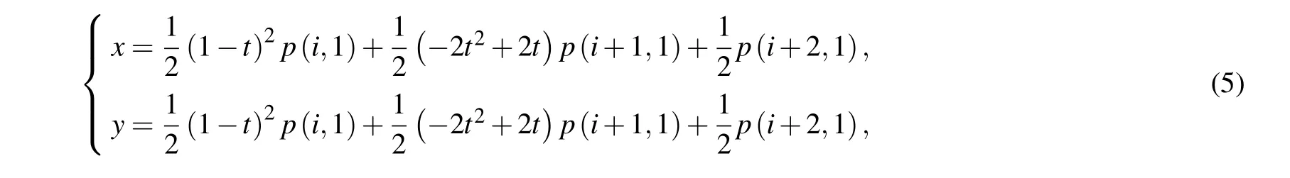
where i is the number of the points, t is a proportional value in a range between 0 and 1,and p is an N-by-2 array of node coordinates.

For the boundary of the geometric domain obtained by the above method, it is necessary to determine the internal boundary when generating the finite element mesh, which fully meets the needs of solving the differential equation with discontinuous material coefficient. The internal boundary divides the whole finite element solution domain into several subdomains, which are connected only by common nodes on the common edge. Generally speaking, a bottom-up method is often used,that is,before the whole domain is meshed,the boundaries are meshed separately,and the positions of the generated nodes and boundary elements are fixed. This method relies heavily on artificial factor, and there is room for further improvement in intelligence and efficiency. In this paper,the implicit distance function is used to represent the internal boundary, and this function is used to project the internal boundary points. The method is slightly different from the previous one, since there are nodes on both sides of the internal common edge, and in this paper the fixed points of the internal boundary are presupposed. In the subsequent iterative optimization process,these fixed nodes are tracked in the direction perpendicular to the inner boundary edge, and the tolerance deps = 0.5h0(h0denotes the initial mesh size) is given. For the newly generated nodes that meet the deps criteria, if they try to cross the boundary, they will be added to the list of boundary nodes and projected on the boundary. The expression is indicated as follows:

where p is the newly generated node which meets the deps criterion, piis the fixed point of the internal boundary edge,fd is the distance function,and p(x0,y0)is the internal boundary node after projection processing. It is important to note that additional quality control is required to avoid overlapping mesh elements.

3.2. Identification algorithm for the location of nodes in polygon area

By introducing fixed points and boundary checking algorithm based on crossing number, Persson’s algorithm determines that the points are located in the polygon region, and the points are inside, outside or on the boundary. A simple implementation requires checking each boundary intersection of each point, resulting in O(N×M) complexity. In order to improve the efficiency of node position state identification,in this paper we propose to estimate the number of segments of the data obtained from the image to the boundary,and segment according to the endpoint of the segmented line chart. Then,starting from the first vertex that intersects the x range of the boundary, the location can be found by the search algorithm,and the piecewise distance function is abstracted based on the coordinates of the head and tail nodes of the boundary,so that the position can be identified and the search process can be terminated when the x coordinate of vertex is beyond the x range of this segment.In the search algorithm,the selection of keynodes as the basis of division is crucial to the efficiency of the entire search algorithm.In this paper,the formula for selecting the keynodes of the record in the middle is updated as follows:

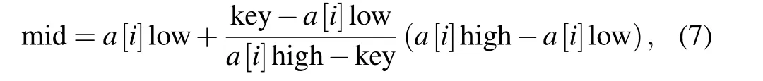
where a[i]can be a segment obtained according to image processing,i represents the number of segments,‘low’and‘high’denote the head and tail data of each segment,and‘key’is the node that needs to identify the position. For the look-up table with large table length and uniform keynodes distribution,the average performance of the data search algorithm is better.

3.3. Novel force-based mesh smoothing algorithm

Appropriate mesh smoothing algorithms can optimize the quality of generated meshes and improve the efficiency of mesh generation. The Persson’s algorithm only describes the repulsive force to help distribute the nodes to the entire Ω domain,but it is inevitable to be iterated frequently.In this paper,a novel force-based mesh smoothing algorithm is proposed,which regards the mesh as a spring-like deformable medium.The whole process can be divided into two stages: measurement of the quality of each element and the average quality of the overall mesh; mesh smoothing operation based on mesh quality.

For the first stage, the mesh quality calculation method is introduced. In the finite element applications, the quality measure of the triangular element mesh can be regarded as the quality measure of the geometric element, which can be calculated in the following way: the upper limit of error depends on the minimum angle in the mesh. To quantify mesh quality,the commonly used quality measure is the relationship between the maximum inscribed circle radius and the minimum circumscribed circle radius,that is,

where a,b,and c are the side lengths. According to the rule of thumb, if the qminvalues of all elements are greater than 0.5,the mesh is favorable.

It is worth noting that in Persson’s algorithm, the force balance state is achieved by fine-tuning the position of mesh vertex. After a certain number of mesh iterations, when the fine-tuning moving distances of all internal nodes are less than the set convergence accuracy, the algorithm must be terminated. Since the quality of the mesh in the mesh generation may already meet the finite element calculation requirements,using the convergence accuracy as the termination condition in the original Persson’s algorithm may cause additional iterations. A threshold value of mesh quality is set as the termination criterion of the proposed mesh generation algorithm.When the quality values of all meshes are greater than 0.5,the mesh generation algorithm will be terminated,which will effectively avoid excessive mesh iteration.

This function only has a repulsive force in mesh smoothing. If the distance between two vertexes is too close,they will repel each other.For the situation that the distance between vertexes may be far away,the function does not consider it,which may cause unnecessary iteration. In order to avoid extra iterations,in this paper we consider giving each bar an attractive force or a repulsive force when performing mesh smoothing iteration.

According to f(sij), with s=1 as the boundary, when s ∈(0,1),the value of the constructed function is greater than 0 and less than 1;when s=1,the value of the constructed function is equal to 0, which conforms to the principle of forcebased smoothing function, in order to satisfy the smoothness of the following constructed function and be close to f(sij),the preliminary construction is f(s)=(1-s2); when s ＞1,the value of the constructed function is less than 0, and approaches to 0 before s=2,which is more in line with the size requirements of the generated mesh.

Based on the above requirements,in this article,we combine f(sij)and use the exponential function as the basis for description,and then we use f(sij)function curve as the boundary to spread points appropriately, and conduct the curve fitting experiments In order to try to construct several eligible smoothing functions as shown in Fig.1.

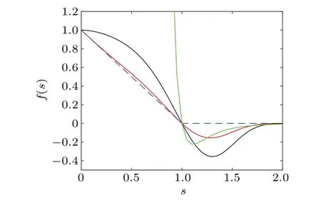
Fig.1. Several curves of smoothing function f(s), with blue line denoting the results from Persson’s algorithm, red line representing (1-s)exp(s3-s4), black line referring to (1-s2)exp(s3-s4), and green line indicating s-13-s-7.

The blue dotted line in Fig. 1 represents the smoothing function adopted by Persson’s algorithm,which only has a repulsive force; the green line is f(s)=s-13-s-7, for mesh generation purpose,this model suffers numerical instabilities,since f(0+)→∞.Performing the iterative tests on the smoothing function represented by the red and black lines,in this article we find that a smoothing function f(s)=(1-s2)exp(s3-s4) with this attraction/repulsion behavior can produce better results. If two nodes are too close to each other, they repel,and if too distant,they attract. This is different from Persson’s smoothing where nodes always repel each other regardless of distance.

Then,a novel smoothing function is constructed based on f(s)=(1-s2)exp(s3-s4). The novel smoothing function(NSE) Eq. (11) constructed in this paper has both repulsion and attraction, in addition, the smoothing function can accurately constrain the magnitude of the force in the smoothing process through quality monitor. After experimental verification, the function is numerically stable, this will allow the smoothing process to proceed steadily. Specifically, the NSE is expressed as

In order to reach a static state,the algorithm in this paper will be iterated through Eq. (12) to update the node position.In Eq. (12), the bar force is applied to a vector of length eij,eijbeing the desired edge length, and Niis the neighborhood of node i.

Fig. 2. (a) Ideal triangle shape, (b) schematic diagram of smoothing function.

Fig.3. Algorithm flow chart.

As shown in Fig. 2(b), mesh smoothing is performed.When the distance between two vertexes in a triangle element of the mesh is too close,s ＜1,the NSE will exert a repulsive force on the bar formed by connecting the two vertexes;when the distance between the two vertexes is far, s ＞1, the NSE will give bar attractive force. Since the NSE can generate an attractive force or a repulsive force according to the value of s, when it is used for the entire mesh, the repulsive force or attractive force on the edges of adjacent meshes will produce mutual assistance and can reduce the adjacent mesh iteration time, which will reduce the overall mesh iteration time. And the applied force is limited based on the mesh quality, which will avoid generating the extremely poor quality meshes.

The process of mesh smoothing proposed in this paper is as follows. After Delaunay mesh generation is ended, the mesh quality is measured;then according to the quality of the mesh, each element performs a corresponding mesh smoothing. For each element, a set of nodal forces preserves the global topology in order to transform the element itself into the best element,and the displacement constraint at the boundary of the domain should be selected correctly.

4. Numerical examples and application

The following tests are for verifying the effectiveness of the proposed algorithm for improving the mesh generation algorithm.

Experimental conditions: computer configuration is as follows:

Intel(R)Core(TM)i5-7500 CPU@3.40 GHZ

4.1. Alpha Lake of Marcus Garvey

The more complex Alpha Lake of Marcus Garvey is taken as the test case. This area is of a polygon with one polygonal hole. Due to the limitations of the conditions, the image of Alpha Lake is taken from the image provided in the Distmesh.In order to facilitate the gray processing,the surface of Alpha Lake is filled with black as shown in Fig.4(a). Without being processed by the path optimization algorithm, the image extraction is shown in Fig.4(b),the fit between the boundary of the image and the boundary of the geometric domain is obviously not high;after the path optimization algorithm is used,it can be seen from Fig.4(c)that the image boundary extraction algorithm based on path optimization can improve the fit.

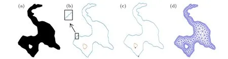
Fig. 4. Alpha Lake (h0 =10). (a) Gray image. (b) Geometric contour map based on boundary extraction algorithm. (c) Geometric contour map processed by path optimization algorithm. (d)Effect diagram of mesh generation.

To test the influence of identification algorithm for locating the nodes in polygon area and the NSE smoothing function on Persson’s algorithm, for the visualization requirements of Alpha Lake meshing, take h0=10, 9, 8, 7, where h0is the initial defined mesh size.

As shown in Table 1, the number of iterations required to optimize the mesh to reach a steady state using the NSE smoothing function is about 50% of the number of iterations required for Persson’s algorithm,and the overall mesh generation speed is increased by 40%.

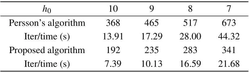
Table 1. CPU time(in unit s)(composite geometry).

The average mesh quality and the minimum mesh quality generated by the Persson’s algorithm are compared with those generated by the proposed algorithm(h0=10),and the results are shown in Tables 2 and 3,respectively.

As shown in Table 2,the average quality of the mesh generated by the proposed algorithm is roughly the same as that by the Persson’s algorithm,all being above 0.8. It can be seen from Table 3 that the mesh quality generated by the Persson’s algorithm is usually high,but the mesh quality will sometimes be low because of the instability of the algorithm. The proposed algorithm performs well in this respect and ensures that the qminis more than 0.5.

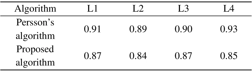
Table 2. Average quality of generated mesh.

Table 3. Minimum quality of mesh generation.

4.2. TEAM workshop problem 30A

The proposed algorithm is then applied to the numerical solution of the TEAM workshop problem 30A. The TEAM problem 30A is to simulate a three-phase induction motor.The physical parameters are given in Fig.5(a).[22]The winding in the stator is excited at a frequency f =60 Hz. The rotor is made of steel (with electric conductivity σ =1.6×106S/m)and aluminum(with electric conductivity σ=3.72×107S/m), with the rotor steel surrounded by the rotor aluminum. The stator steel is laminated and its conductivity is set to be σ =0.

Fig.5.(a)Setting of TEAM workshop problem 30A.(b)Gray image.(c)Geometric contour map based on boundary extraction algorithm.(d)Geometric contour map processed by path optimization algorithm. (e)Mesh for TEAM workshop problem 30A.(f)Flux density and flux lines at 600 rad/s.

Fill the Fig. 5(a) with equal difference RGB values.On the basis of gray processing, the image adaptive Multithreshold segmentation (Otsu) is used for gray segmentation,and then the image geometric edge is extracted by image edge detection technology. It can be seen from Fig. 5(c) that the extracted geometric boundary is not smooth,which may have a limited influence on the accuracy of finite element analysis.Through the boundary smoothing algorithm based on the path optimization proposed in this paper, the extracted geometric edge is smoothed and optimized as shown in Fig. 5(d). Obviously, the smoothness of geometric boundary is improved,which helps to improve the accuracy of mesh generation. Finally,using the mesh generation algorithm proposed in this paper,the mesh generation graph is shown in Fig.5(e). It can be seen from the figure that the performance of the inner boundary processing method adopted in this paper is outstanding,and the inner boundary is in a smooth state.

It can be seen from Table 4 that after the introduction of the NSE smoothing function, the number of iterations of the algorithm is about 50% of the Persson’s algorithm’s, and the running speed is increased by 50%. Comparing with the common meshing algorithms Gmsh,the speed is about 20%higher than that of the Gmsh. The mesh quality obtained by the proposed algorithm is stable. Comparing with the original algorithm,the mesh quality has not decreased significantly.

Table 4. Results obtained by different algorithms.

Then the finite element boundary information obtained by the proposed algorithm is applied to the numerical solution of TEAM workshop problem 30A. Let NArepresent the turns’density for the phase winding in Fig.5(a),where the current in the phase winding is indicated. Using a similar nomenclature for phase windings and B and C windings, Fourier space decomposition can write the current density of three-phase winding as

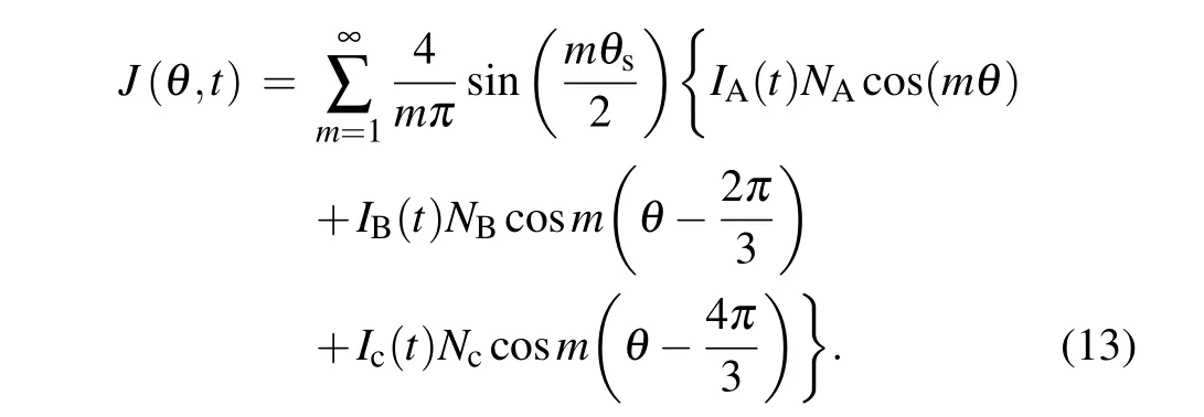
Assume that the three phases have the traditional time harmonic distribution, each phase with the same current density IN,then we will have

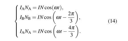
Using Euler’s rule to represent the cosinusoidal dependence,equation(13)can be written as

where

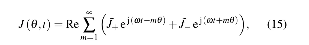
In this form, it is clear that the three-phase winding yields two counter-rotating waves. In a single-phase machine,equation(15)may take the following form:

where

The problem of Fig.5(a)consists of multiple piecewise homogeneous regions.The solution can be developed in each region by using the transfer relation concept given by Melcher.[23,24]In nonconducting regions,the magnetic vector potential is assumed to have a coulomb gauge dependence and satisfies the Poisson’s equation

Then,by using the finite element method in the time domain to solve the following time-domain eddy current equation represented by Euler’s formula and homogeneous Dirichlet boundary conditions, the magnetic field in TEAM workshop problem 30A three-phase induction motor can be simulated. The flux density and flux line of 600 rad/s in Fig. 5(f) can be obtained by solving the following equation:

Taking the center of motor as the origin of coordinate system,the unit coordinate length is 1m. The following four points are selected to verify the flux density: P1: (0.0151, 0.0131),P2: (-0.0283, 0.0131), P3: (-0.0534, -0.0122), and P4:(0.0510,-0.0214),which are shown in Table 5.

Table 5. Influences of different algorithms on solution of potential.

By obtaining random points from the results of commercial finite element software and combining the numerical values solved by the proposed algorithm,a clear comparison can be made to prove the correctness of the algorithm calculation results. Comparing the times taken by the four finite element solution methods,it can be seen from Table 5 that the finite element processing based on this algorithm is about 20%more efficient than commercial software. Comparing with the finite element processing based on Persson’s algorithm, the time is reduced by 50%;comparing with Gmsh,the speed is increased by 20%.

5. Conclusions

Two-dimensional unstructured mesh generation based on Persson’s algorithm is proposed for calculating the electromagnetic field in this paper. The numerical results demonstrate that compared with the original Persson’s algorithm and commercial software,the algorithm can generate high-quality meshes in the solving domain, the iteration time is reduced by about 50%, and comparable solutions can be obtained in electromagnetic calculations. As the structures of electromagnetic devices become more complex,electromagnetic models are built in three dimensions to obtain a precise solution.In the future work the authors will focus on improving the efficiency of mesh generation in three-dimensional problems.