Boling Guo,Shuyan Chen

(Institute of Applied Physics and Computational Mathematics,Beijing 100088,PR China)

Abstract

Keywords inverse scattering;Riemann-Hilbert problem;long-time asymptotics;initial value problem(IVP);initial boundary value problem(IBVP)

1 Introduction

In 1967,Gardner,Greene,Kruskal and Miura(GGKM)proposed the inverse scattering method.It’s the most effective method for the exact solution of the IVPs for the nonlinear evolution equations whose initial values decay sufficiently rapidly,through a series of linear equations rather than by linearized perturbation method.We will obtain the more direct and clearer picture of the solution by the inverse scattering method,which is different from the conventional energy method of nonlinear partial differential equations,for example,the method helps to get the behaviors of t→ ∞ or x→ ±∞ for the Korteweg-de Vries(KdV)equation,the nonlinear Schr¨odinger equation(NLS)and so on.Meanwhile,the inverse scattering method as a new method is used to prove the regularity of the solution.Many scholars have done a lot of excellent work in this field in recent years[13–21].This paper briefly introduces the research status and recent progress in this field.

2 The Inverse Scattering Method and the IVP for the KdV Equation

In this section,we briefly introduce the inverse scattering method for the exact solution of the IVP for the KdV equation.

For the Burgers equation

using the Hopf-Cole transformation

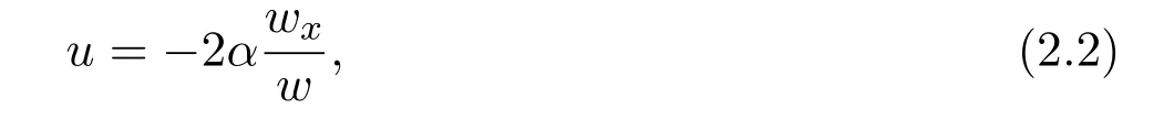
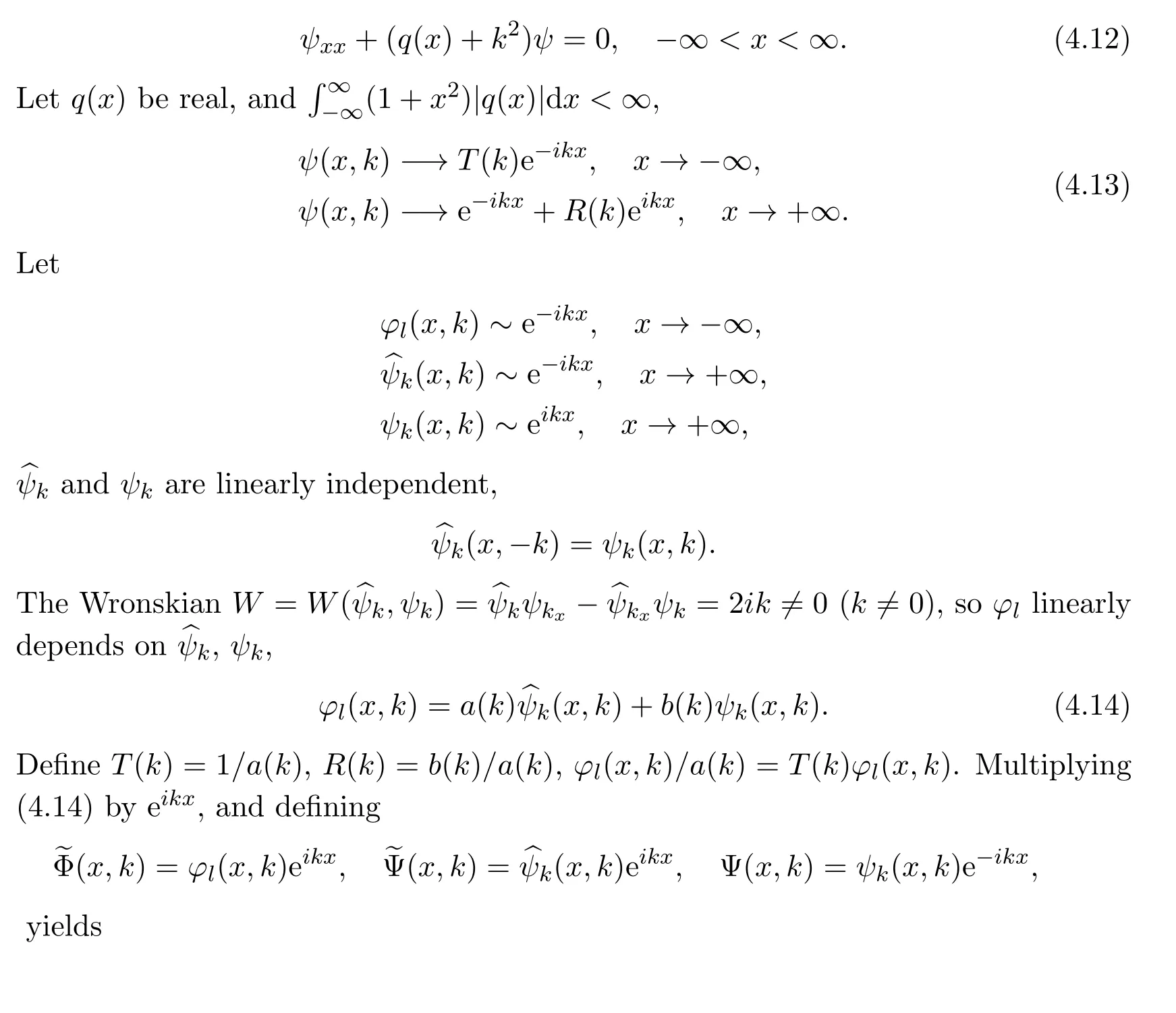
it can be converted to a linear thermal conductivity equation about w

and the original equation has the solution

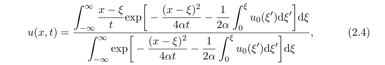
where u0(x)is the initial condition,u|t=0=u0(x).

In 1952,E.Hopf proved that(2.4)tends to the generalized solution of quasilinear hyperbolic equation(ut+uux=0)as α → 0,and the basic theory of quasilinear hyperbolic type theory was established accordingly.For other nonlinear partial differential equations,it’s hard to reduce them to linear partial differential equations.

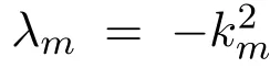
In 1967,GGKM found a new precise method for the exact solution of the IVP for the complete integrable KdV equation through a series of linear equations.Consider the KdV equation

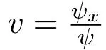
where ψ is the wave function,u is the potential,and λ is the energy spectrum.

Fixed t,define the solution of scattering problem(2.6)satisfying the boundary conditions(shown in Figure 1)

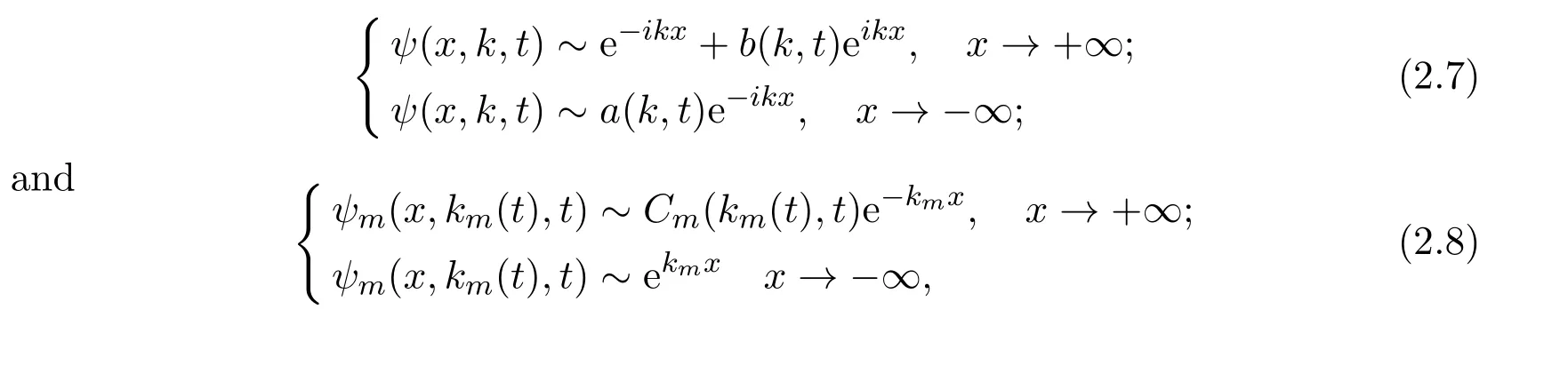
Figure 1

where b(k,t)is the reflection coefficient,a(k,t)is the transmission coefficient,Cmis the attenuation factor and

Direct problem:At time t=0,u(x,0)solves the direct scattering problem,that is,given the scattering datas km,b(k,t),a(k,t),Cmat time t=0,can obtain the wave function ψ.

Inverse Problem:Using the scattering data to reconstruct the potential u(x,t).The relation about the potential u(x,t)and scattering data may be summarized as follows.

The potential is reconstructed by the relation

where K satifies Gel’fand-Levitan-Marchenko equation

whose kernel is defined by

which are respectively the sum for the discrete spectrum and the integral for the continuous spectrum.

Obviously,the above relation(2.10)not really complete the inverse scattering method.In order to determine the potential u(x,t),K must be determined,but the K is decided by the scattering datas such as Cm,km,a(k),b(k),these datas are resolved by the potential u(x,t).This creates an endless cycle.We introduce the following theorems to break the cycle.

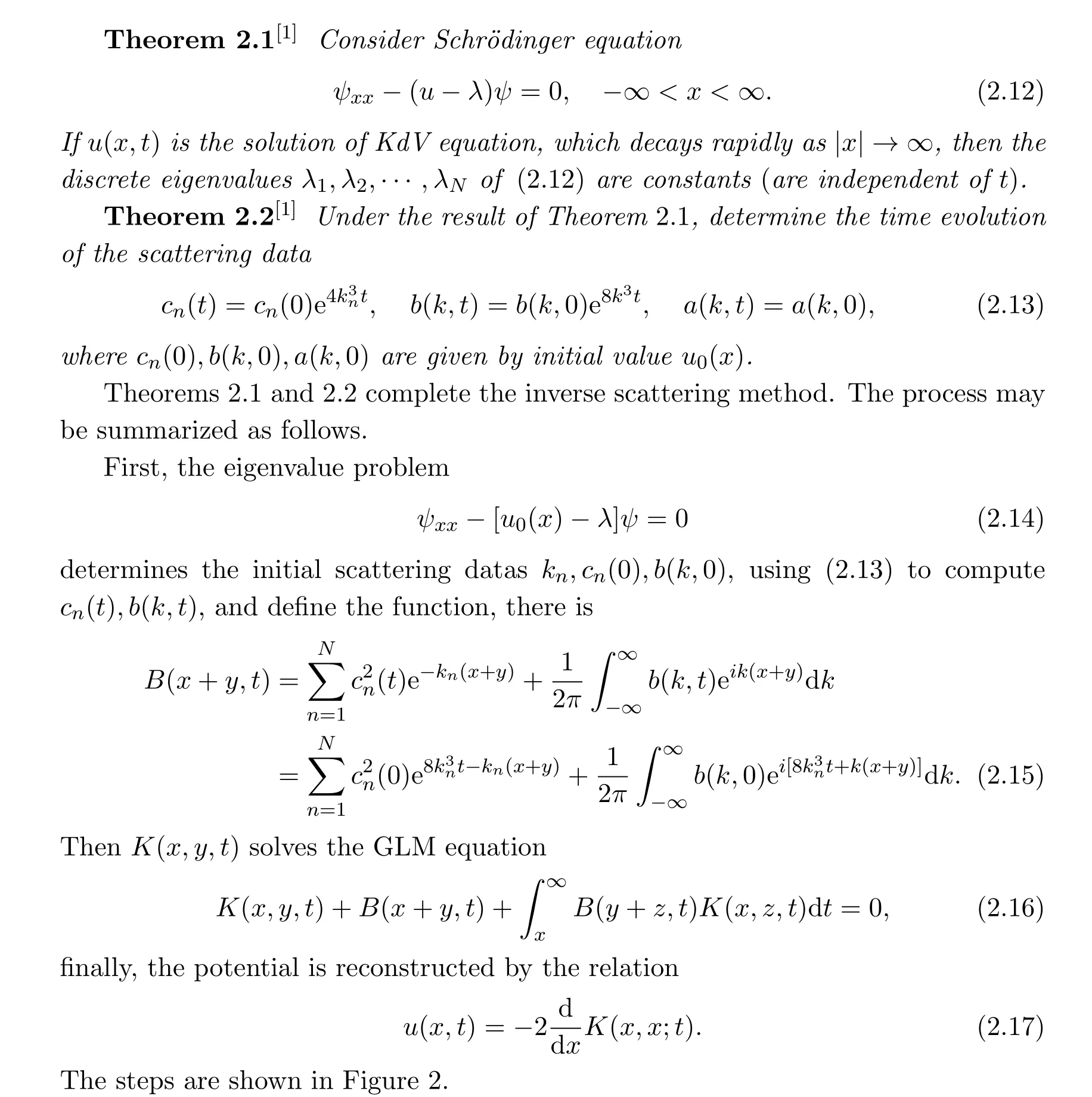
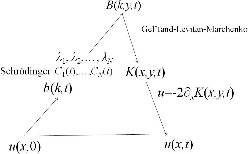
Figure 2

Thus,reduce the IVP for the nonlinear equation(the KdV equation)to a problem of solving two linear equations.One is Sturm-Liouville problem for the second order ordinary differential equation,the other is to find a solution for the linear integral equation.Next we give two examples to illustrate it.

Suppose that u0(x)=2sech2x,using hypergeometric functions to solve the eigenvalue problem of(2.14)exactly.It has a discrete eigenvalue k1=1.The normalization constants are given byThe GLM equation

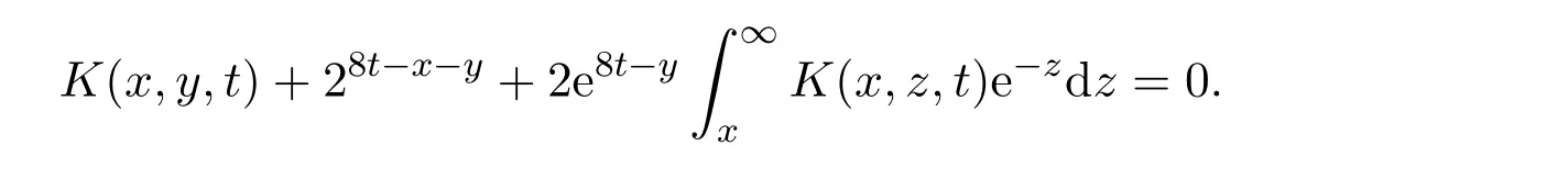
Assume that K(x,y,t)has the form K(x,y,t)=L(x,t)e−y,this yields

It is easy to verify that K(x,y,t)is the only solution of the GLM equation.Thus we have the solution of the KdV equation

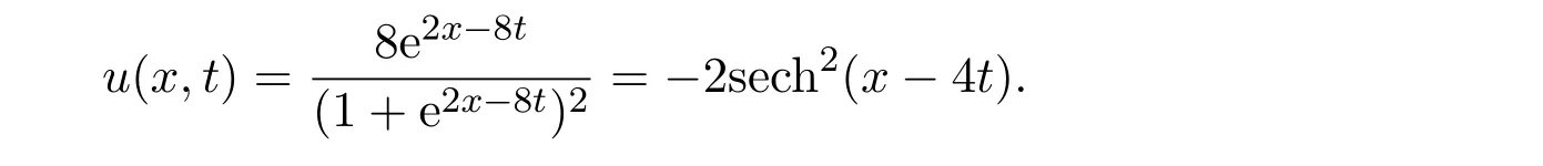
The traveling wave solution shows that it is indeed an exact solution of the IVP for the KdV equation.

For another example,suppose that u(x,0)=u0(x)=−6sech2x,there have two different eigenvalues k1=2,k2=1.b(k,0)=0 yields

The inverse scattering method can be used to solve the N-soliton solution for the KdV equation or the other one dimensional and higher dimensional complete integrable equation,such as AKNS integrable system.

3 Long Time Asymptotics

In this section,we introduce two methods to deal with the asymptotics evaluation of integrals(also used in solving the Riemann-Hilbert problem),and give the long time behaviors of the KdV equation as a example.

Definition 3.1[2](The Method of Steepest Descent)Consider the large k asymptotics of integrals of the form

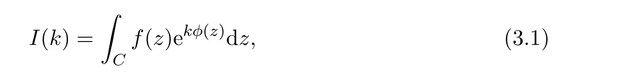
where C is a contour in the complex z plane and f(z)and ϕ(z)are analytic functions of z.The basic idea of the method is to utilize the analyticity of the integrand to justify deforming the contour C to a new contour C′on which ϕ(z)has a constant imaginary part.Thus if ϕ(z)=u+iv,the integral I(k)becomes(Imϕ =v=constant)

Paths where v is a constant are also paths for which the decrease of u is maximal.A point z0for which ϕ′(z0)=0 is called a saddle point.Consider a single path of steepest descent originating from a saddle point ϕ(z0)of order n − 1.Assume that f(z)is of order(z−z0)β−1near z0,that is,as z → z0

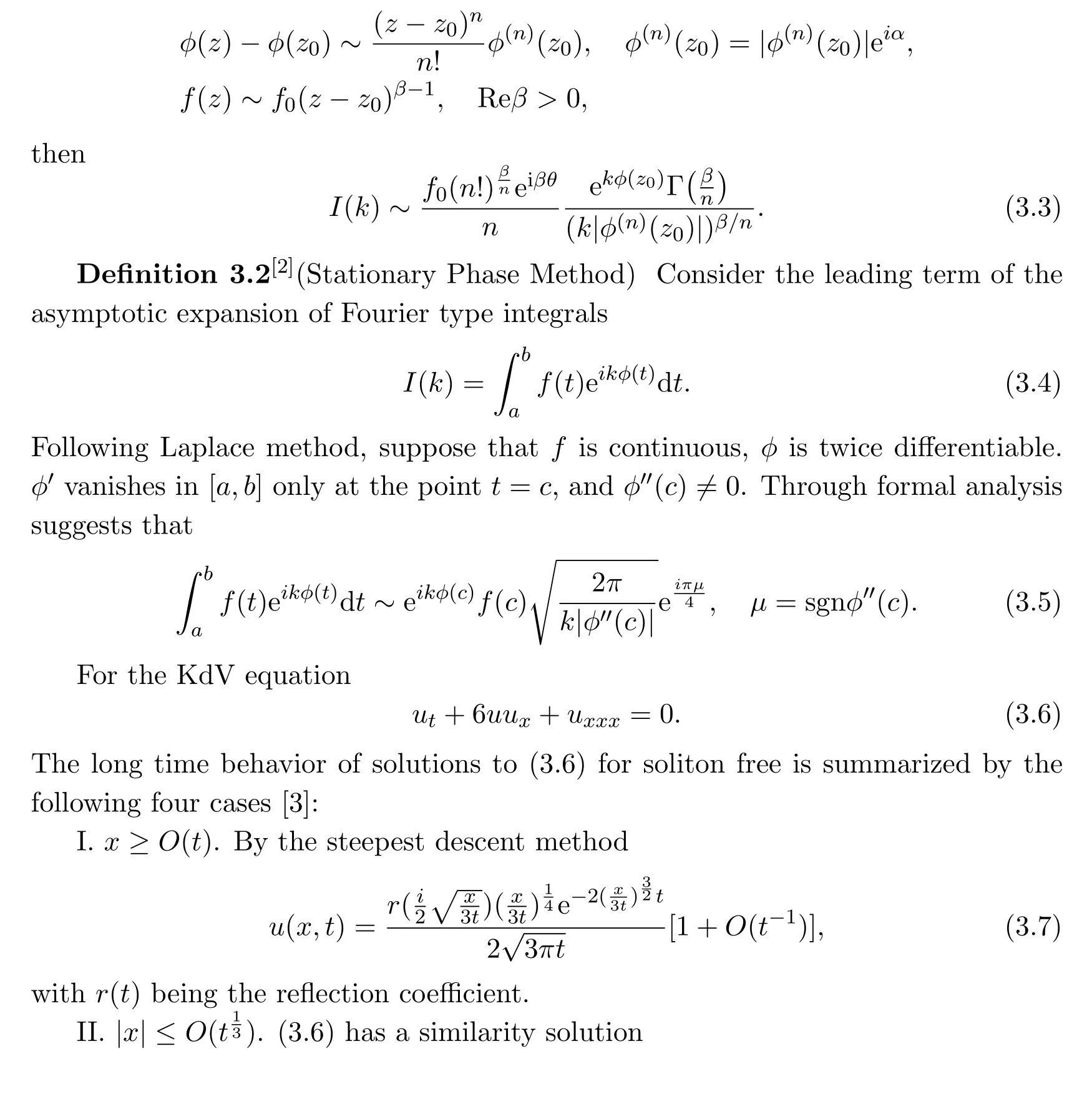
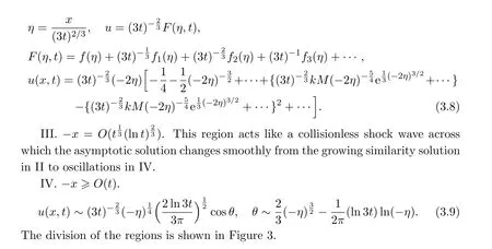
Figure 3

4 Riemann-Hilbert Problem

In this section,we introduce the definition of the scalar(matrix)Riemann-Hilbert problem,and obtain the exact solution or long time asymptotics of the IVPs for the NLS equation,mKdV equation,and KdV equation.

Consider the integral

where L is a smooth curve(L may be an arc or a closed contour)and φ(z)is a function satisfying the H¨older condition on L,that is for any two points τ and τ1on L,

If λ =1,the H¨older condition becomes so-called Lipshitz condition.

Lemma 4.1[2]Let L be a smooth contour(closed or open)and φ(τ)satisfy H¨older condition on L.Then the Cauchy type integral Φ(z),defined by(4.1),has the limiting values Φ+(t)(as z approaches L from the left)and Φ−(z)(as z approaches L from the right),and t is not an endpoint of L.These limits are given by

where Lεis the part of L that has length 2ε,and center around t.As depicted in Figure 4.

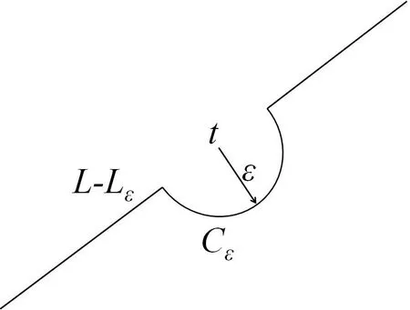
Figure 4

The scalar homogeneous Riemann-Hilbert(RH)problem for a closed contour[2]:

where Φ±(t)are the boundary values of Φ(z)on C.Assume that the index of g(t)is κ.

The solution of this RH problem with Φ(z)with degree m at infinity and the index of g(t)being κ is given by

where Pm+κ(z)is an arbitrary polynomial of degree m+κ≥0,and X(z)called the fundamental solution of(4.5)is given by

with κ=indg(t)on C.

The matrix RH problem for a closed contour C is defined as follows[2]:

Given a contour C and an N×N matrix G(t)that satisfies a H¨older condition and is nonsingular on C(that is,all the matrix elements(G)ijsatisfy H¨older condition,and detG(t) ̸=0 on C),find a sectionally analytic vector function Φ(z)(column vector),with finite degree at infinity,such that

Suppose that X(z)=(X1(z),X2(z),···,XN(z))Tis the fundamental solution of(4.9),and

1)在涂有W3.5金刚石研磨膏的铸铁上将焊件试样接头部位磨平，分别采用W3.5及W1.5的金刚石研磨膏将试样在抛光机上抛光，以抛光面上无明显划痕为宜。

Any solution of the homogeneous RH problem is given by

where P(z)is an arbitrary polynomial vector,that is,each component of P(z)is an arbitrary polynomial.

The relation between the solution q(x)and the matrix RH problem is as follows.

The NLS equation with potemtial q(x)is

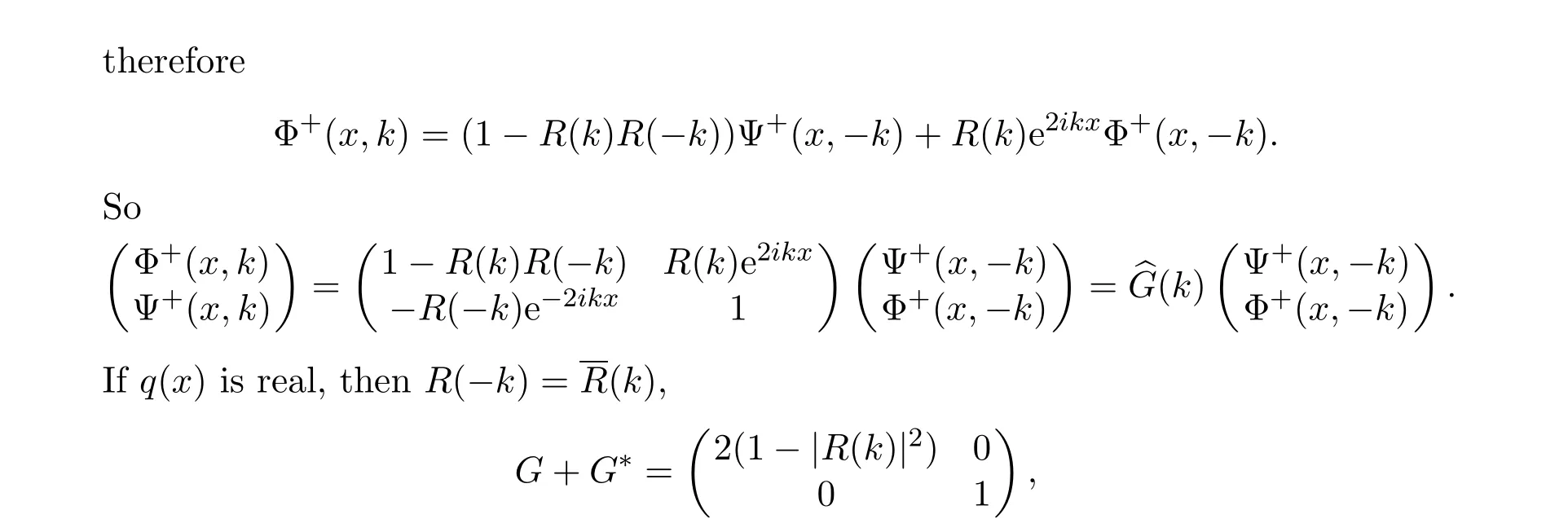
further if|R(k)|＜1,G+G∗is positive definite,the RH problem is solvable.

4.1 Long time behaviors for solutions of the mKdV equation

Consider the IVP for the modified Korteweg-de Vries(mKdV)equation

In 1993,P.Deift and X.Zhou[5]evaluated the long-time behavior of the mKdV equation by the inverse scattering method,the steepest descent method and stationary phase method.For each t＞0,the ODE operator is

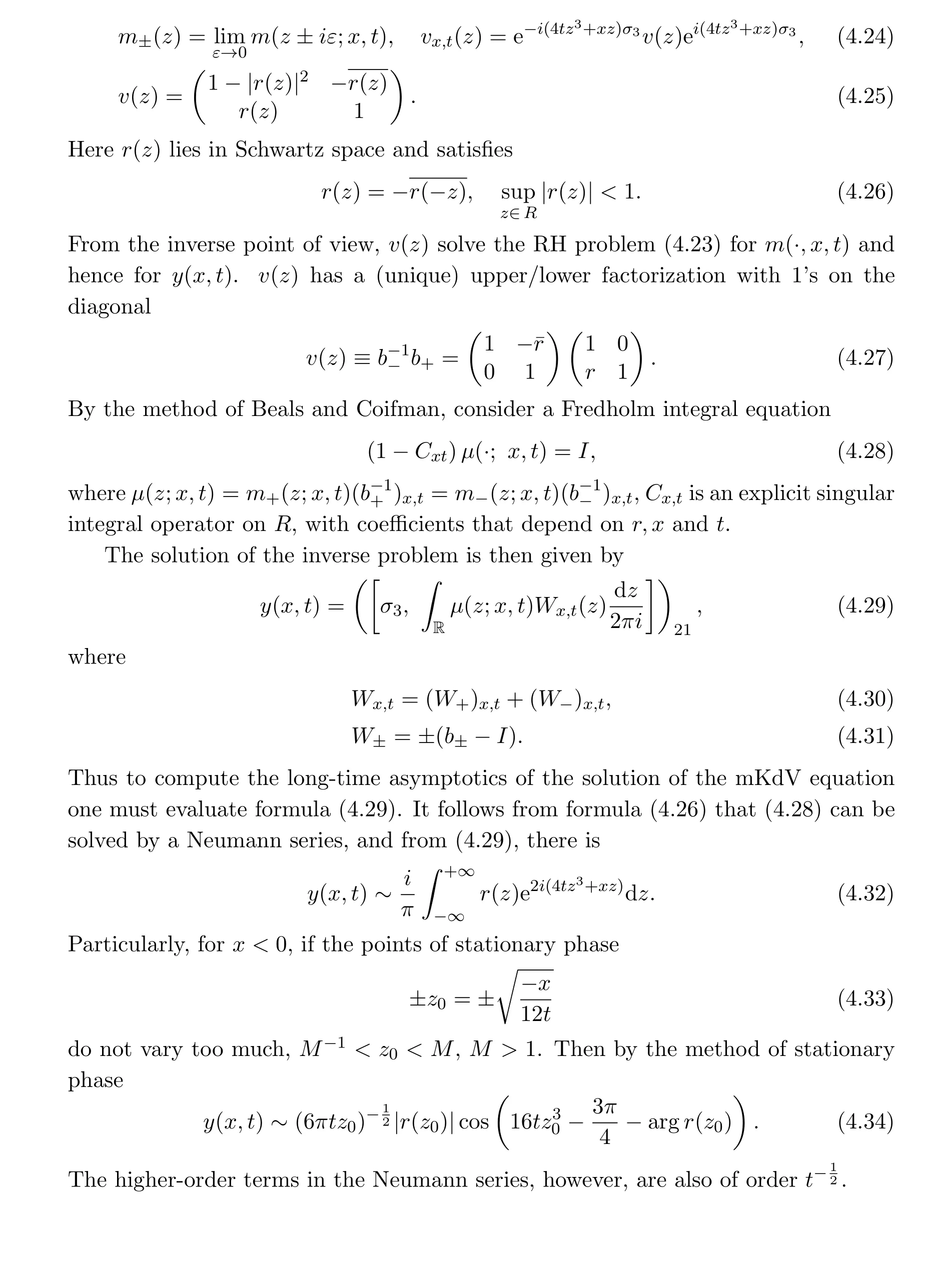
Directly consider the RH problem(4.23).By deforming contours in the spirit of the classical method of steepest descent,one show how to extract the leading asymptotics of the mKdV equation.In the standard inverse problem at fixed t,say t=0,one must show that the solution y(x,0)constructed from formula(4.29)decays rapidly as x→ ±∞.For x→ +∞,the critical role is played by the upper/lower factorization v(z)(4.27).Using the Fourier transform,one writes,

where h1(x,z)decays rapidly as x→+∞for z∈R,whereas,hz(x,z)has an analytic continuation to Imz＞0,which is bounded and converges to 0 as z→∞and decays exponentially as x→+∞,consequently if we set

where

The decay of y(x,0)as x→−∞ can now be inferred from(4.42).

In the long-time asymptotic problem,when t is variable,it is no longer possible to decompose

where,h1,h2rapidly decay as t→∞,and are uniformly bounded in Imz＞0.

The crucial observation is that the complex plane must be decomposed according to the signature of Re(iF)(F=(4tz3+xz)).For x＜0,the signature is shown in Figure 5.

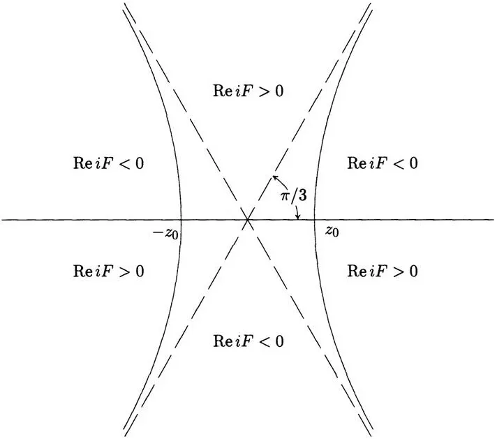
Figure 5

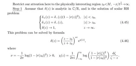
Step 4As t → ∞,the interaction between ΣA′and ΣB′goes to 0 to higher order and the contribution to y(x,t)through equation(4.23)is simply the sum of the separate contributions from ΣA′and ΣB′.

Figure 8

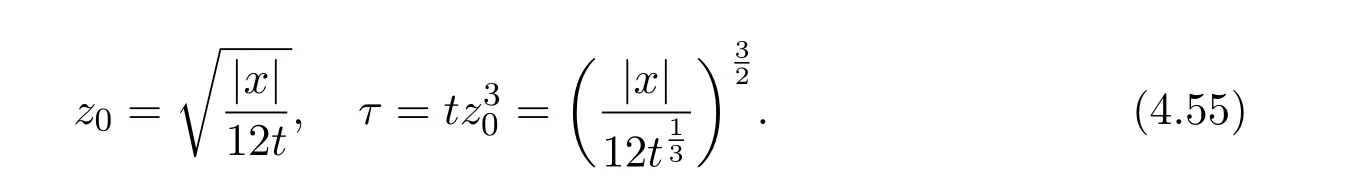
Define M and M′to be fixed constants greater than 1.

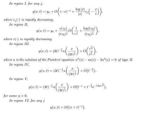
Theorem 4.1[5]Let y0(x)lie in a Schwartz space,the reflection coefficient is r(z).As t→∞the solution y(x,t)of mKdV equation,with initial data y0(x),has uniform leading asymptotics converniently described at fixed(t≫1),in the six regions shown in Figure 9.

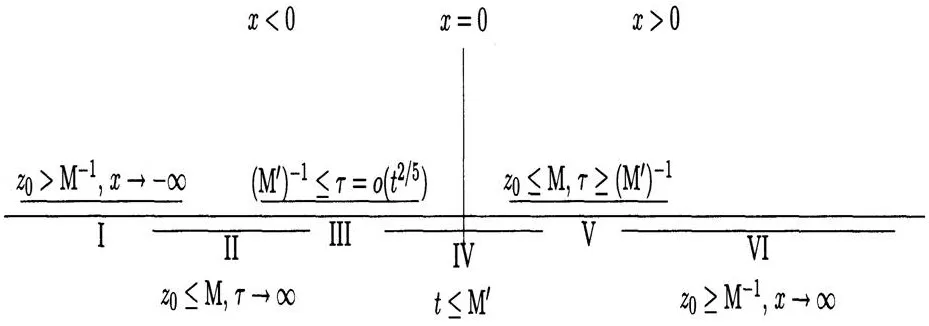
Figure 9

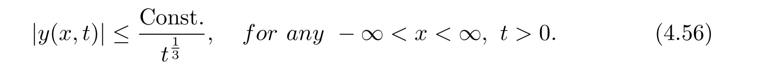
The above results imply the global asymptotic stability of the zero solution of mKdV in the sup norm.More precisely is shown in the following corollary:

Corollary 4.1[5]Let y(x,t)be the solution of the Cauchy problem for the mKdV equation with Schwartz-space initial data.Then

4.2 Long time behaviors for solutions of the defocusing NLS equation

Within the framework of the inverse scattering method,[6]studied the long time asymptotics for the solutions of the defocusing NLS equation

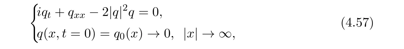
4.3 Existence and regularity for solutions of the KdV equation

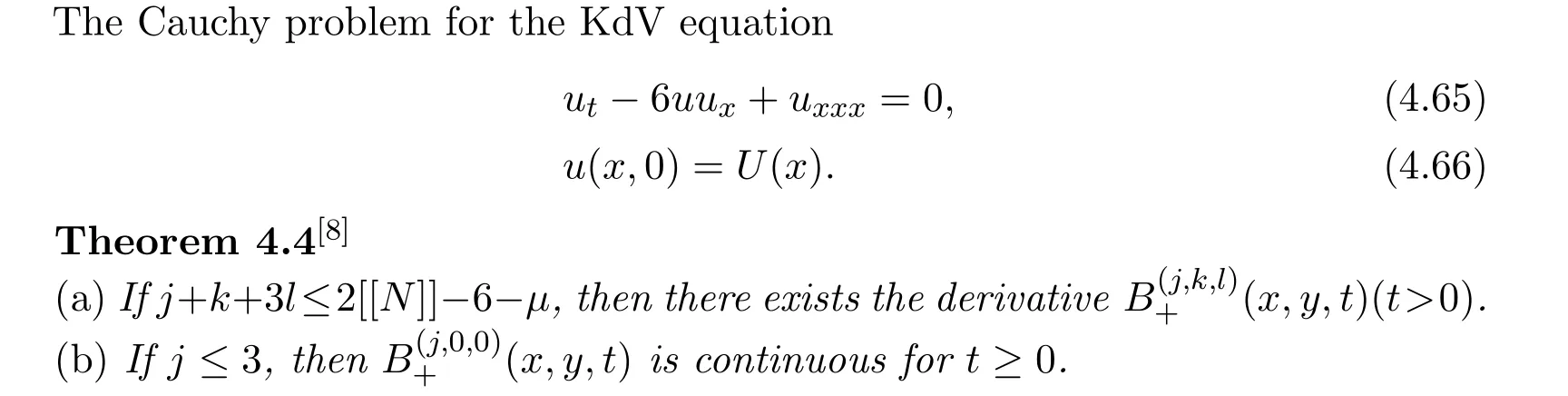
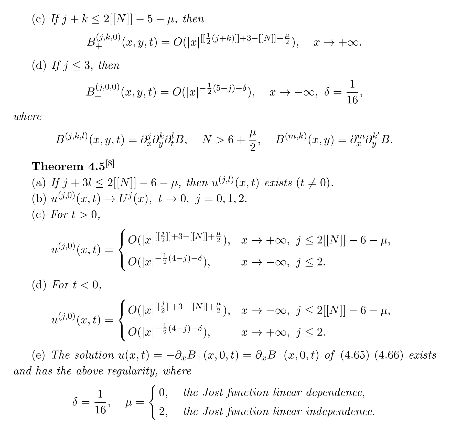
From(4.7),if t＜0,x→ +∞,u rapidly decays.But as x→ −∞,it slowly decay.

In the next section,we introduce the application of the inverse scattering method to IBVPs,which yield the relation of the potential and the solution of a RH problem.

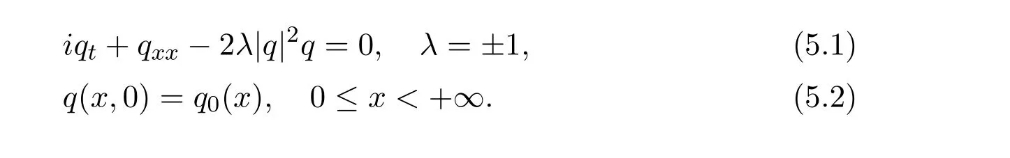
5 The Inverse Scattering Method and the IBVP for the Integrable System

5.1 IBVP on the half line

Fokas in[10]researched the IBVP for the NLS equation

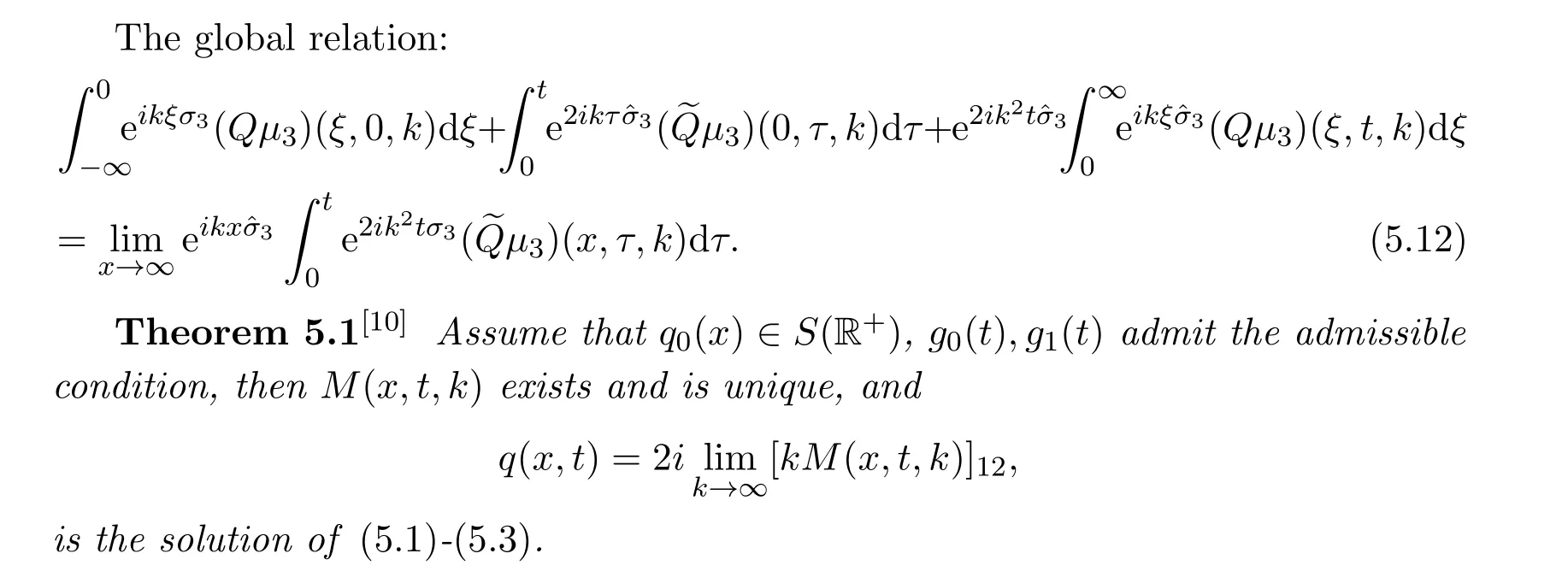
For the IBVP on the half line,how to use the solution M(x,t,k)of the new RH problem to express the solution q(x,t)of the equation?Fokas used the scalar function a(k),b(k),A(k),B(k)to express,where a(k),b(k)are determined by q0(x)=q(x,0),and A(k),B(k)are determined by g0(t)=q(0,t),g1(t)=qx(0,t).These spectral functions are not independent and satisfy the global relation.

(5.1)admits a Lax pair formulation of the form

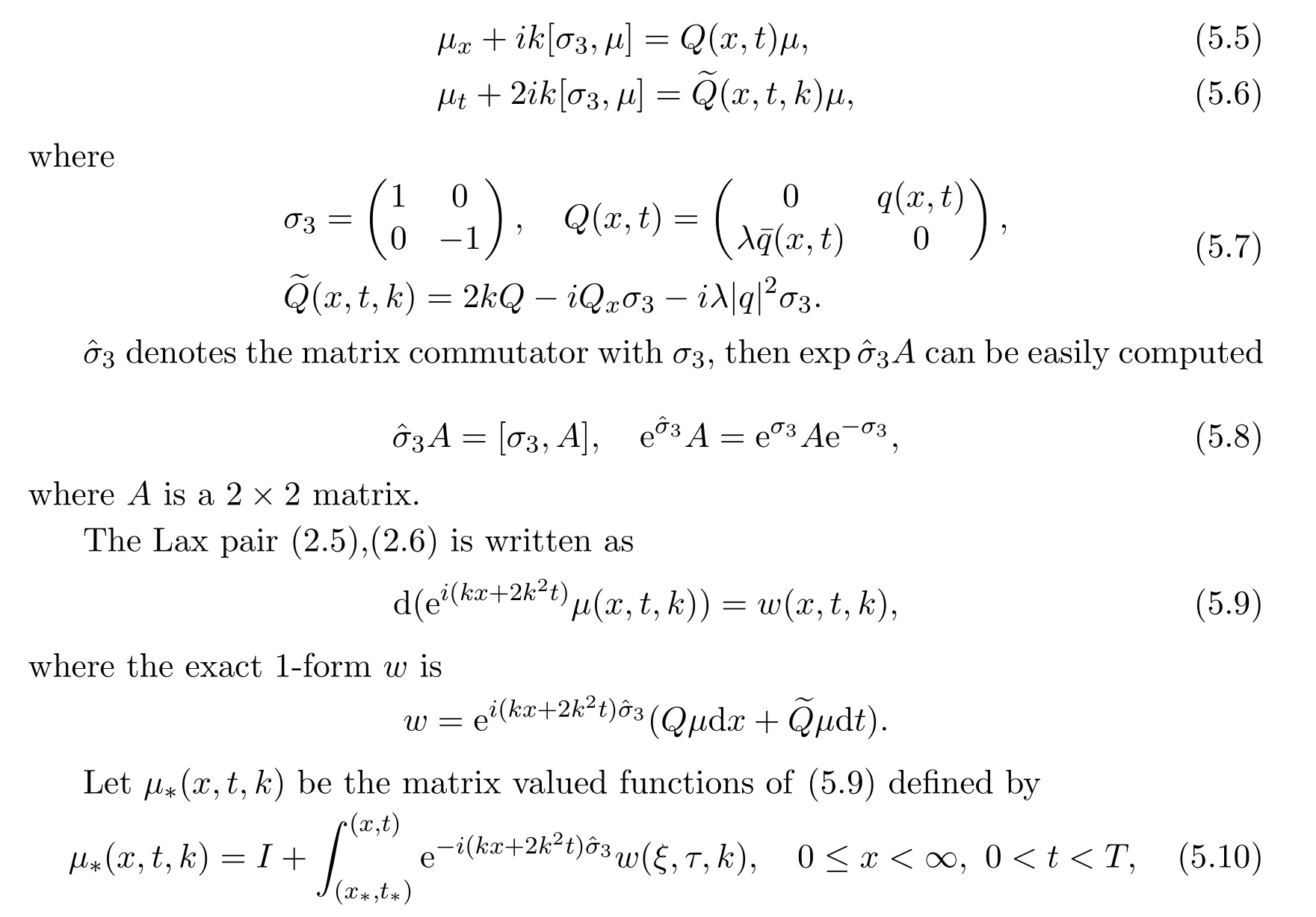
where I is a 2×2 identity matrix.(x∗,t∗)are any point in 0＜ ξ＜ ∞,0＜ τ＜ T.The integral is a smooth curve derived from(x∗,t∗)to(x,t).Due to w exact 1-form,µ∗is independent of the path of the integral,choosing starting point(x∗,t∗)as the collection of the vertices of this polygon.the three corners are the points(0,T),(0,0),(∞,T).µ1,µ2,µ3are the eigenfunctions corresponding to these corners.Typical contours are shown in Figure 10.

Figure 10:(a)µ1:(0,T),ξ−x≤ 0,τ−t≥ 0,Imk≤ 0,Imk2≥0.(b)µ2:(0,0),ξ−x≤0,τ−t≤0,Imk≤0,Imk2≤0.(c)µ3:(∞,T),ξ−x≥0,Imk≥0.

Let k=a+bi,k2=a2−b2+2abi,and the analysis of the second column element ofµ1,µ2,µ3,are shown in Figure 11.

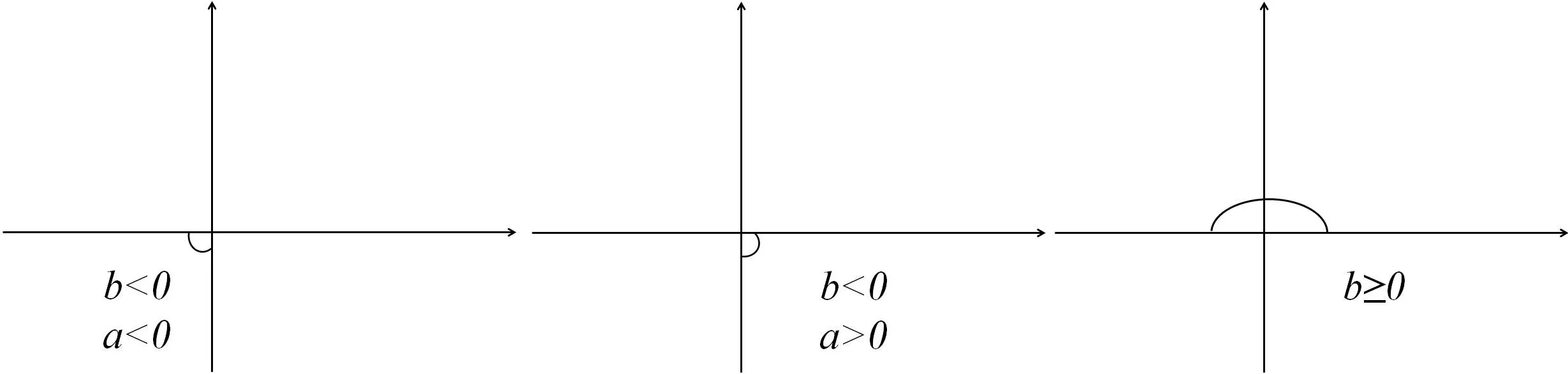
Figure 11

Similar study the analysis of the first column element of µ1,µ2,µ3.The superscripts(1,2,3,4)will denote the domain of analyticity of the relevant vector eigenfunction:

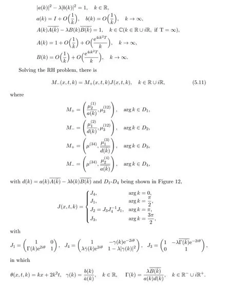
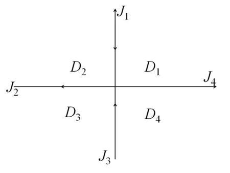
Figure 12

5.2 IBVP on the interval