Lingfeng LU(卢凌峰),Ying LIU(刘莹),Huizong DUAN(段会宗),Yuanze JIANG(姜元泽),2 and Hsien-Chi YEH(叶贤基)

1 TianQin Research Center for Gravitational Physics and School of Physics and Astronomy,Sun Yat-sen University(Zhuhai Campus),Zhuhai 519082,People’s Republic of China

2 MOE Key Laboratory of Fundamental Physical Quantities Measurement & Hubei Key Laboratory of Gravitation and Quantum Physics,PGMF and School of Physics,Huazhong University of Science and Technology,Wuhan 430074,People’s Republic of China

Abstract

Keywords:plasma turbulence,gravitational wave detection,laser interferometry

1.Introduction

Since the first ground detection of gravitational waves(GWs)by the Laser Interferometer Gravitational-Wave Observatory(LIGO)team in 2015[1],scientists have moved on to GW detection in space,which has a frequency band distinct from ground detection.Laser Interferometer Space Antenna(LISA)[2],Taiji[3]and TianQin[4]are among the well-known ongoing spaceborne GW detection programs.

TianQin is a gravitational wave observatory[4],to be launched around the year 2034.Three geocentric and circularly orbiting spacecraft will construct an equilateral triangular constellation,aiming to detect GWs in the frequency band of millihertz.The radius of the spacecraft orbit is 105km,corresponding to 15.62RE(REis the radius of the Earth).Each spacecraft pair will therefore establish a 1.7×105km long laser arm.Figure 1 shows the variations of the TianQin orbit,following the revolution of the Earth.The GW detection periods are from June to September and December to March in each year.During these two periods,the Sun-Earth line is almost perpendicular to the detection plane,which avoids light contamination in the telescopes from solar radiation.The detection plane is designed to point at a well-chosen GW source,a whitedwarf binary,RX J0806.3+1527.When a GW passes the TianQin constellation,due to the polarizations of the GW,one arm will observe periodical expansion and contraction,while the other experiences the converse.The spaceborne GW detectors adopt the same principle as ground-based GW detectors[5]:making use of laser interferometry to measure tiny variations of the distances in-between the three spacecraft.Each spacecraft pair contains two counter-propagating laser links.The variation of the path length is detected by measuring the phase deviation of the laser beams.Unlike ground-based detection,GW detection in space is carried out in an environment that also contains space plasmas.

Figure 1.Orbital view of the TianQin constellation.Letters A-D specify the approximate dates dividing detection periods from non-detection periods.

Laser beam tracking and acquisition is conducted when establishing the inter-spacecraft laser link.At this stage,the precise alignment of the laser beams is performed by measuring the wavefront of the received laser beams.This sets a criterion for the flatness of the wavefront[4]:after propagating 1.7×105km in space plasma,the wavefront arriving at the receiving telescope(hereafter called the receiver)should not vary by more than 10−6rad,compared to a wavefront that propagated the same distance in vacuum.The spacecraft are located at the interface between the solar wind(SW)and the magnetosphere,see section 4 below.There are plenty of large-scale waves in this area,e.g.ultra-low-frequency(ULF)waves[6].These perturbations can cause plasma turbulence leading to wavefront distortion of the laser beams,and thus affect GW detection[7].Therefore,it is necessary to analyze the effects of plasma turbulence on the laser’s wavefront.To the knowledge of the authors,no literature has so far been published discussing the effects of wavefront distortion due to space plasmas by either of the spaceborne GW detection programs.This effect is probably more significant for TianQin than for LISA and Taiji,since TianQin adopts a geocentric orbit,whereas the other two follow a solar orbit,thereby making themselves immune to the variations of the space environment in the magnetosphere.On the other hand,choosing a geocentric orbit makes it possible to use sophisticated models and relatively abundant in situ measurements to analyze and survey the space environment throughout the TianQin mission.

Regarding laser propagation in turbulent media,the reader is referred to the earlier work on the study of the interactions between laser beams and atmospheric turbulence.In the atmosphere,laser beams can encounter stochastic small scale perturbations which lead to variations in the beam’s phase and radiance.This phenomenon is called scintillation,[8]and it is often characterized by a scintillation index.The conventional way to calculate the scintillation index is to solve the scalar wave equation by adopting the Rytov perturbation theory,and then construct multilayer phase screens to model the phase modulation of the laser beams by the turbulent medium[9,10].This is the so-called weak fluctuation theory.It assumes that the perturbation is small compared to the averaged background.However,the plasma density in space can often change by one or two orders with respect to the background density.Andrews et al[11-13]recently further extended the Rytov perturbation theory to moderate and strong turbulences.Schmidt[14]used the split-step beam propagation method to model laser propagation in atmospheric turbulence,which has been widely used in adaptive optics.A dedicated Matlab function has been developed accordingly,to tackle the interactions of laser beams with atmospheric turbulence[14].

All the literature mentioned above solves the simplified wave equation or the scalar wave equation.This is valid when the refractive index or the permittivity of the turbulent medium is a scalar and there is no charge source or loss inside the turbulent medium.

Previous literature[15,16]has demonstrated that even though the temperature of the space plasma around the TianQin orbit could often reach hundreds of eV,it could still be described by the cold plasma approximation given the laser frequency.Using the cold plasma approximation,the plasma permittivity is described by the Stix dielectric tensor[17],

where S,P and D are components of the Stix tensor with the following expressions,

andωpeis the electron plasma frequency,

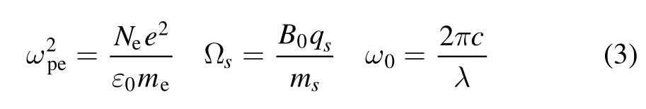
where Neis the plasma density,ε0is the vacuum permittivity,meis the electron mass,e is the unit electrical charge,qsis the electrical charge of species s,B0is the background magnetic field strength,c is the speed of light and λ is the wavelength of the laser beams.

The TianQin constellation uses neodymium-doped yttrium aluminum garnet(Nd:YAG)continuous lasers with a wavelength of 1064 nm and an electric power of 4 W.Following the orbit of the spacecraft,the laser beam in-between two spacecraft will pass through the bow shock,the magnetosheath,the magnetopause and the inner magnetosphere.Given the typical plasma parameters at those regions,i.e.the major ion species H+,O+and He2+,a plasma density of 106m−3,a magnetic field ofB0=10 nT,an electron temperature ofkBTe=100 eV(where kBis the Boltzmann constant)and a laser frequency ofω0=1.88×1015rad s−1.With these parameters,the cold plasma dielectric tensor(1)can be reduced to a scalar,i.e.The wave equation in the plasma is thus,

Using the constitutive relation,the LHS of Poisson’s equation reads,

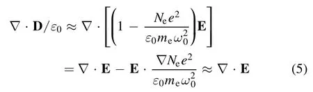
where we have used an estimation of the density fluctuation in space,i.e..The plasma Debye length is about 70 m(Ne=106m-3,kBTe=100 eV).Since we are considering laser propagation at a very large scale,i.e.1.7×108m,charge neutrality could still be well preserved.Thus,

The underlying assumption in equation(6)is that we ignore the effects of the electromagnetic field induced by charge separation within the Debye length on the laser’s propagation.In fact,since the plasma density is about one particle in 1 cm3,the electromagnetic field induced by such low density particles should be extremely weak.

Substituting(6)into(4),the wave equation in plasma could be simplified as the following,

This is critical,since our model is based on the scalar wave equation,as will be emphasized in the next section.In addition,both the power spectra of turbulence in space plasmas and in the atmosphere follow certain power laws[10,18,19].Based on these facts,we applied the atmospheric turbulence-laser interaction model to the space plasma.

The structure of this paper is as follows:section 2 is the theoretical basis of the atmospheric turbulence-laser interaction model.Section 3 gives the verification of the adopted model.Section 4 predicts the realistic phase distributions at the receiver for the given orbit of TianQin.Section 5 presents the conclusions.

2.The theoretical basis of the atmospheric turbulence-laser interaction model[10,14,20]

Laser propagation in a stochastic medium is described by the scalar wave equation.Any of the three components of the electric field fulfills

where k is the wave number,n is the refractive index,r is the position in the reference frame and E is the electric field component.When the inhomogeneity of the medium is much larger than the laser wavelength,the scalar wave equation can be further simplified to the parabolic equation.Assuming the laser propagates in the z direction,the parabolic equation reads

where n1is the deviation of the refractive index from its mean value and ∇⊥is the gradient perpendicular to the direction of propagation.Solving the parabolic equation,one can get the field component U,which stands for any of the x,y or z components of the vectors E and B.U is a complex number.It contains the phase and the amplitude of the laser beam.As shown in figure 2,one could separate laser propagation in a turbulent medium into laser propagation in vacuum and phase modulation by turbulence.By adopting two partial propagation methods[14],U can be expressed as,

where R is the diffraction operator,T is the refractive operator,ziis the z position of the ith phase screen,riis the distance from the center of the ith phase screen to the objective point and Δziis the distance from the ith phase screen to the(i+1)th screen.In a vacuum,T=1,whereas in the turbulent media,

where Φ(ri+1)is the phase modulation by the turbulent media in the ith phase screen.Equations(9)-(11)are the fundamentals of modeling laser propagation in a stochastic medium.The phase modulation of the phase screen can be written as a weighted sum of basis function,either using Zernike polynomials or a Fourier series.Making use of a Fourier series,the phase modulation reads,

wherecn,mis the coefficient of the Fourier series,andfxnandfymare the discrete spatial frequencies in the x and y directions,respectively.According to the central-limit theorem,the complex valuecn,mshould follow a Gaussian distribution.Both the real and imaginary parts ofcn,mshould have a zero mean and equal variances.cn,mcan be expressed as,

where〈〉refers to the average,ΔfxnandΔfymare the inverses of the grid sizes in the x and y directions and Φφ(f)is the phase power spectral density(PSD)of the atmospheric turbulence.The Kolmogorov or modified Von Karman phase PSD is commonly used to describe the stochastic turbulence.For example,the modified Von Karman phase PSD reads[14,21],

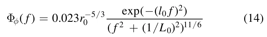
where L0is the turbulence’s outer scale,l0is the turbulence’s inner scale and r0is the atmospheric coherence diameter.is the amplitude of the spatial frequency in polar coordinates.

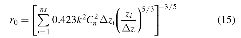
where ns is the number of phase screens andis the refractive index structural parameter,measured in m−2/3.

In the simulation,we first calculate the mean value ofcn,mby(13),then multiply a number of computer-generated random numbers by the zero mean and the unit variance to obtaincn,m.After that,the phase modulation at each phase screen can be obtained by(12).

3.Numerical tests of the atmospheric turbulencelaser interaction model

This paper uses the Matlab code developed by Schmidt[14].To ensure the reliability of the code,a few tests were made,as described in this section,before conducting the simulations required to meet our needs.The tests started with laser propagation in a vacuum and then moved on to turbulent media.The model uses dedicated point sources since,in our case,the distance between two spacecraft is large enough to consider the laser emitter(20 cm in diameter)as a point.Besides,a laser beam emitted from any extended object can be well represented as the weighted sum of a series of point sources.One can therefore model a realistic laser source without any large modifications to this code.

3.1.A test of laser propagation in a vacuum with different point sources

As a first step,we tested laser propagation in a vacuum.Laser beams emitted from two types of point sources were compared,in order to select the better source for the rest of the simulations.The two point sources are the Sinc and Sinc-Gaussian point sources,respectively,as used by Schmidt[14].The diameter of the receiver or the region of interest in the observation plane was 8 mm,the wavelength was 10-6m and the propagation distance Dz=1 km.The laser beam propagated in the z direction and the origin of the coordinate was the center of the source plane.

Figure 3 shows the irradiance of the source and observation planes for the two kinds of point sources.The abscissa represents the cut line at y=0 of the corresponding planes.Figure 3(a)shows that the side lobes of the irradiance decrease slightly with the Sinc-Gaussian point source.In figure 3(b),the irradiance from both two point sources fits well at the center of the region of interest.While the irradiance of the Sinc-Gaussian source decreases smoothly at the edge of the region of interest,the Sinc source has abrupt changes.Figure 4 illustrates the phase simulations versus the theoretical predictions in the observation plane for the two point sources.The phases from both sources fit well inside the region of interest.While the Sinc point source has numerical noise outside the region of interest,the Sinc-Gaussian source behaves well in the whole observation plane we selected.Overall,the Sinc-Gaussian source is more compatible with the model and we will keep using this point source in the following simulations.

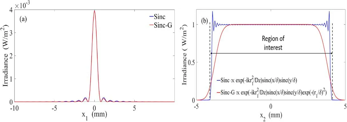
Figure 3.(a)The irradiance distributions in the source plane for Sinc and Sinc-Gaussian point sources.(b)The irradiance distributions for these two sources in the observation plane.The expressions of the Sinc and Sinc-Gaussian point sources are shown.Dz is the propagation distance,δ is the width of the point source.

Figure 4.(a)A comparison of the phase simulation and its theoretical prediction for the Sinc point source.(b)A comparison of the phase simulation and its theoretical prediction for the Sinc-Gaussian point source.

3.2.A test of laser propagation through a turbulent atmosphere

After testing laser propagation in a vacuum,the Sinc-Gaussian point source was selected and applied in the following tests of laser propagation in a turbulent atmosphere.The parameters used in the simulation here are the following:the propagation distance in atmosphere was 50 km,the diameter of the region of interest in the observation plane was 0.5 m,there were eleven identically distributed phase screens,l0=0 m,L0=Inf.The other parameters are the same as those used in figures 3 and 4.Figure 5 compares the irradiance and the phase distributions of laser beams propagating in the observation plane for the cases of propagation in vacuum and in turbulent atmosphere.These results are consistent with Schmidt’s simulations[14].

When modeling laser propagation in turbulence,the wave structure function[14,22]and the coherence factor[14]are the typical indicators for illustrating the statistical properties of the turbulence.The detailed expressions for these two quantities can be found in the appendix.Figure 6 shows the results of the tests of the wave structure function and the coherence factor in the observation plane.The simulation results for the coherence factor and the wave structure function are based on(A.1)and(A.2),while the theoretical predictions are derived from(A.3)and(A.4).To obtain the simulation results of the coherence factor through the mutual coherence function,20 plots of U at each phase screen were generated and then averaged.As shown in figure 6,the simulation results were very close to the theoretical predictions,indicating that the phase screens were set up correctly and that the model can represent laser propagation in turbulent media fairly well.

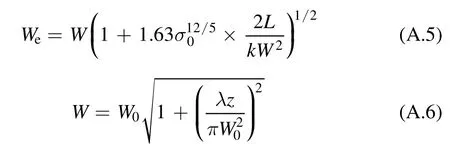
In order to double-check the simulations in a turbulent atmosphere,we finally conducted tests on the effective spot size.The theoretical prediction and the numerical calculation of the effective spot size can be obtained by(A.5)and(A.7),respectively.In this simulation,we used the same parameters as Qian did in her work[23]:the wavelength is 6.328×10−7m,the propagation distance is 1 km,the initial radius of the beam waist is W0=60 mm,l0=1 mm and L0=10 m.Figure 7 illustrates the numerical value and the theoretical prediction of the effective spot size.These two values are very close,with a relative error of less than 2.5%.Figure 7 matches with Qian’s result[23].

Figure 5.A comparison of irradiance and phase in the observation plane between laser propagation in a vacuum and in a turbulent atmosphere.(a)The irradiance distribution for laser propagation in a vacuum,(b)the phase distribution for laser propagation in a vacuum,(c)the irradiance distribution for laser propagation in a turbulent atmosphere,(d)the phase distribution for laser propagation in a turbulent atmosphere.

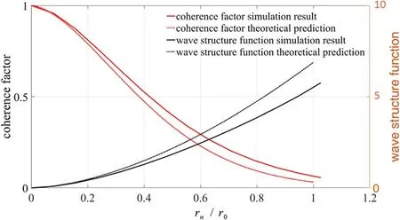
Figure 6.Simulations of the wave structure function,the coherence factor and their theoretical predictions for laser propagation in a turbulent atmosphere.

4.Modeling of laser propagation in turbulent plasmas for TianQin’s GW detection

This section uses the atmospheric turbulence-laser interaction model to conduct realistic simulations for laser propagation in turbulent plasmas within the space environment of TianQin.Before revealing the laser’s phase distribution after propagating 1.7×105km in space plasma,one has to determine the characteristic parameters of the tubulence,e.g.the refractive index structural parameter,the inner scale l0and the outer scale L0of the plasma turbulence.The turbulence’s scale length can be obtained by a spectral analysis of the plasma density along the laser propagation path.Thus the spatial distributions and temporary evolution of the plasma density are needed along the laser arms.Since no in situ measurement can provide such detailed density data,the sophisticated plasma density model known as the Space Weather Modeling Framework(SWMF)[24]is used.This model needs real-time solar wind data at the model’s boundary and the realistic spacecraft orbit data as inputs.In return,it produces the general space plasma data,i.e.the realtime density distribution.In this work,the input solar wind data is projected from the Advanced Composition Explorer(ACE)spacecraft to the simulation box inflow boundary at x=33REand the orbit of the TianQin constellation takes advantage of the earlier work on orbit design and optimization based on the General Mission Analysis Tool(GMAT)software[25,26].

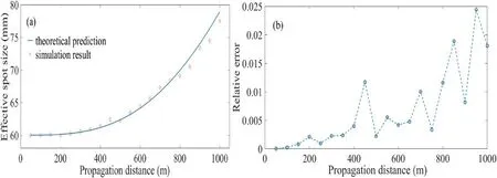
Figure 7.(a)A numerical calculation of the effective spot size versus its theoretical prediction.(b)The relative errors between the simulation and theory.

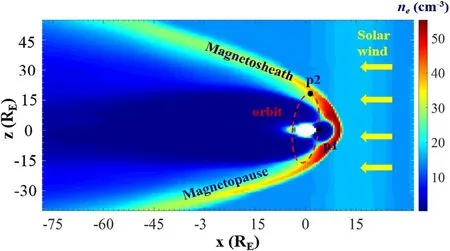
Figure 8.A view of the plasma density distribution in the x-z plane,y=0.The data selected were from 06:00 UT on Aug-10-2000.The schematic configuration of the TianQin constellation’s orbit is shown in red dashed circle.Points 1 and 2 indicate two positions where the temporal variation of the plasma density is examined in figure 9.

Figure 8 gives an example of the magnetospheric plasma density distribution obtained from the SWMF model through the Community Coordinated Modeling Center(CCMC)platform[27],which shows the plasma density at 06:00 UTC on Aug-10-2000.The red dashed circle represents the orbit of the TianQin constellation at that moment.The figure adopts the geocentric solar magnetospheric(GSM)coordinates,in which the origin is the center of the Earth,the x axis points from the Earth to the Sun and the z axis is the projection of the Earth’s magnetic dipole(positive north)on the plane perpendicular to the x axis.

Real-time solar wind data rely on in situ measurements.That is to say,we could not predict the space weather in the year 2034 right now,due to a lack of input data.Instead,in this section,a real minor magnetic storm(Kp=5)which took place from 05:20 to 09:20 UT on Aug-10-2000 is selected,to roughly represent space weather on Aug-10-2034.This specific data is chosen because the Sun-Earth line on this day was nearly perpendicular to the TianQin orbital plane,and thus can well indicate the real space environment during the detection period,i.e.the period of AB in figure 1.The plasma density at two selected points from the TianQin orbit and the solar wind data are depicted in figure 9.The temporal resolution of both the plasma density and the solar wind density from the SWMF model is 1 min.One can see that the plasma density variations are in a close relationship with the density oscillations of the solar wind,meaning that the solar wind dominates the plasma density oscillations at those two points.

Figure 9.Temporal variations of the plasma electron density at two selected points in figure 8 and the input solar wind ion density at 33RE.(a)The density at p1 with GSM coordinates(0,15.62RE,0),(b)the density at p2 with GSM coordinates(0,0,15.62RE),(c)the solar wind ion density at(33RE,0,0).The axis is universal time on Aug-10-2000.

Figure 10.(a)The spacecraft positions at 04:00 UT on Aug-10-2034 with the magnetospheric plasma density at 04:00 UT on Aug-10-2000 in the background;the red triangles mark the points where the density is selected to evaluate the refractive index in figures 12 and 13.(b)The plasma density distributions along the three arms at two different moments,04:00 and 05:00 UT on Aug-10-2000,the solid lines correspond to the density distributions at 04:00 UT and the dashed lines refer to the density distributions at 05:00 UT.

The density distribution along the three arms is examined to see which part of the arm experiences the most significant density change.Figure 10(a)shows the positions of the three spacecraft at 04:00 UT on the day of Aug-10-2034 with the density in the background.In each arm,two red triangles mark the positions where the local densities are used in figures 12 and 13.Figure 10(b)evaluates the density distributions along the three laser arms at 04:00 and 05:00 UT on the same day as in figure 10(a).The red dashed line in figure 10(b)links the second and third spacecraft.The density is apparently smaller than the other two at the extremities,which is reasonable since the greater part of this line lies in the inner magnetosphere,whereas both the other two lines cross the magnetosheath.One can also see that the largest temporal variation of density occurs in the magnetosheath.

Figure 11 is a spectral analysis of the plasma density distribution along the arm between the second spacecraft and the third spacecraft using the plasma density distribution at 04:00 UT,i.e.the red solid line in figure 10(b).The amplitude spectral density(ASD)curve includes an inertial subrange in which the density(ASD)decreases linearly.The lower limit of the inertial subrange indicates the outer scale of the turbulence,i.e.L0=2×107m in figure 11.Spectral analyses of the density distributions from the other two arms suggest the same result.The inner scale could not be fixed from figure 11 at this moment due to the limited spatial resolution of the density data.The typical approach is to set l0=0 m.This work only considers large-scale turbulence,such as that induced by ultra-low-frequency waves.Those waves have a wavelength in-between 104m and 108m,which is comparable with the arm length.The implicit assumption here is that we ignore the small scale turbulence,as it may be averaged over the whole laser path.Besides,the mesh size used in the SWMF simulation is about 3200 km at the altitude of 105km,so smaller-scale turbulence is simply not modeled.From figure 11,the spectral index is about -1,corresponding to-3 in 3D.This result is consistent with other literature[18,19].

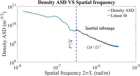
Figure 11.The amplitude spectral density of the plasma versus the spatial frequency.

The turbulence refractive index structural parameter[10]can be determined by measuring the time-averaged difference of the refractive index between two different points located at r1and r2,

where the refractive index at an arbitrary point is a function of the plasma density Neat that point[28]

Each simulation takes about 2 h with the workstation used.Figure 14 is the phase distribution in the receiver’s plane after propagating 1.7×105km in a turbulent plasma.The result for propagation in vacuum remains roughly the same shape.Figure 15 shows the difference of the phase distribution in figure 14 with respect to its counterpart in the case of laser propagation in vacuum.The phase difference is of an order of 10-9rad.Strictly speaking,figure 14 is rather the phase distribution in the plane perpendicular to the z axis,not the wavefront.But with a point source,one can derive the wavefront at the receiver directly from figure 14 by deducting the phase deviation due to the tiny difference of the propagation distance between the points at the receiver and the points at the arrived wavefront.The divergence angle of the laser used in TianQin is less than 10-5rad.Given the width of the spot size is 10 m,the longest path from the arrived wavefront to the receiver is thus about 10-4m.Within such a tiny distance,the plasma effects can be neglected,since the density is very low.Therefore,figure 15 should be equivalent to the wavefront distortion at the receiver.

In practice,provided the divergence angle is 10-5rad,a Gaussian beam emitted from an ideal point source would expand its radius to the order of kilometres after propagating for 1.7×105km.It is this expanded beam width that is critical for spacecraft tracking and acquisition.Therefore,instead of focusing on the tiny region of the receiver,i.e.20 cm in diameter,one would rather be interested in examining the phase distribution at a plane comparable to the scale of the radius of the arrived laser beam.Figure 16 shows the phase distribution at a plane much larger than the diameter of the receiver.The mesh size used in the figure is 10 m,and the number of phase screens is 100;the other parameters are the same as in figure 15.Even at a scale length of 1 km,the phase difference still remains within 10−9rad,which is three orders less than the error budget.Finally,an examination of the dependence of the results on the power spectral index is also conducted.The results show that changing the spectral index to-3 instead of-11/3 as indicated by a modified Von Karman phase PSD does not affect the order of the results in figures 15 and 16.These results suggest that large-scale plasma turbulence should not significantly reduce the sensitivity of the laser interferometer.

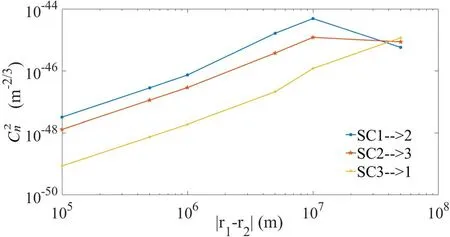
Figure 12. versus the distance between two points on three laser arms,e.g.varying the distance between the two adjacent points marked by red triangles on each arm in figure 10(a),a time interval of 07:00-07:20 UT is selected.

Figure 13. versus time,with a fixed distance of 107 m between the two points on each arm indicated in figure 10(a).

5.Discussion and conclusions

This work reports the preliminary results on the wavefront distortion of inter-spacecraft laser beams due to plasma turbulence in the context of the TianQin GW detection mission.Given the laser frequency and the plasma parameters of TianQin when in orbit,the cold plasma approximation is still valid.The plasma dielectric tensor tends to be a scalar at the high-frequency limit and this provides the precondition for the adoption of the atmospheric turbulence-laser interaction model in tackling our problem.It should be emphasized that this model did not consider the weak electromagnetic field induced by charge separation within the Debye length.The effect of this electromagnetic field on laser propagation is yet to be explored.In addition,the space plasma model and realistic TianQin orbital data are exploited to obtain the characteristic parameters of the plasma turbulence.For TianQin’s inter-spacecraft lasers,the preliminary calculation shows that the wavefront distortion of the laser beam due to turbulent plasmas in the propagation path is in the order of 10-9rad.It will thus not affect the GW detection.This wavefront distortion should be distinguished from the phase deviation calculated by the line integral of the plasma density along the laser’s path.The latter can reach up to 10-5rad during a magnetic storm.The result obtained in this paper merely represent the higher-order correction induced by turbulence.

Figure 14.The phase distribution in the receiver’s plane after propagating 1.7×108 m in a turbulent plasma,with eleven phase screens and a mesh size of 0.1 m.

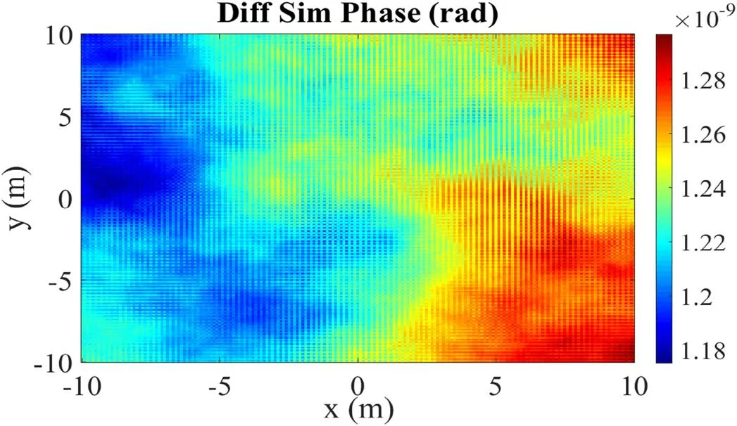
Figure 15.The phase difference at the receiver’s plane between laser propagation in a turbulent plasma and in vacuum.

Up until now,this work has not analyzed the uncertainties of the results due to the SWMF density model adopted.A crude estimation of the phase variation can be made based on(12)-(17),i.e.Thus even if the root-mean-square error(RMSE)of the plasma density from the SWMF model can reach 0.961 compared with the in situ measurements[29],it should not affect the order of the phase distribution obtained.Besides,the calculation is based on a real magnetic storm event,which should already represent the results in conditions of relatively severe space weather.The current calculation neglects the high-frequency part of the density oscillation,due to the limited resolution of the measurement data and the density model.This will be improved when a finer measurement or a more precise model is available.Furthermore,the turbulence spectral analysis needs a stationary random process,while the zone used in the present spectral analysis spans many different regions(solar wind,bow shock,magnetosheath,magnetopause,and magnetosphere),so whether the spectral analysis is applicable or not remains an open question to be investigated.Finally,the calculation relies on the real-time in situ measurement of the plasma data in space,which emphasizes the importance of real-time surveillance of the space environment in the region of the TianQin spacecraft.This work will provide scientific objectives and theoretical guidance for forthcoming spaceborne GW detection experiments.

Figure 16.The phase difference at the receiver’s plane with an extended diameter of 1 km,100 phase screens and a mesh grid at the receiver’s plane of 10 m.The other parameters are the same as in figure 15.

Acknowledgments

The authors wish to thank Dr Xianmei Qian at the Anhui Institute of Optics and Fine Mechanics and Prof.Zhiwei Ma at Zhejiang University for many useful discussions.Some simulation results in this paper were provided by the Community Coordinated Modeling Center at Goddard Space Flight Center through their public Runs on Request system(http://ccmc.gsfc.nasa.gov).The SWMF/BATS-R-US Model was developed by the Center for Space Environment Modeling at the University of Michigan.This work was supported by the China Postdoctoral Science Foundation(No.2018M643286)and the postdoctoral funding project of the Pearl River Talent Plan.

Appendix.Definition of the phase structure function,the coherence factor and the effective spot size

The statistical property of the turbulence is often characterized by the phase structure function and the coherence factor.The coherence factor is defined[14,22]as,

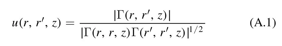
where Γ(r,r′,z)=〈U(r)U*(r′)〉is the mutual coherence function.The wave structure function is linked with the coherence factor by the following expression,

The coherence factor for a plane-wave source with Kolmogorov turbulence can be written[14],

where r is the distance between any two points in the phase screen.According to(A.2),the wave structure function then reads,

Some literature also uses the effective spot size to validate the numerical model.Consider a Gaussian beam with an initial waist radiusW0and a wavelength ofλ.After propagating a distance of L in the atmosphere,the effective spot sizeWeis[11],

where I is the irradiance and r is the distance from the point(x,y)to the mass center of the spot at the phase screen.