Hamed Kazemi and Alireza Yazdizadeh,

Abstract—This study proposes a scheme for state estimation and, consequently, fault diagnosis in nonlinear systems. Initially,an optimal nonlinear observer is designed for nonlinear systems subject to an actuator or plant fault. By utilizing Lyapunov’s direct method, the observer is proved to be optimal with respect to a performance function, including the magnitude of the observer gain and the convergence time. The observer gain is obtained by using approximation of Hamilton-Jacobi-Bellman(HJB) equation. The approximation is determined via an online trained neural network (NN). Next a class of affine nonlinear systems is considered which is subject to unknown disturbances in addition to fault signals.In this case,for each fault the original system is transformed to a new form in which the proposed optimal observer can be applied for state estimation and fault detection and isolation (FDI). Simulation results of a singlelink flexible joint robot (SLFJR) electric drive system show the effectiveness of the proposed methodology.

I. INTRODUCTION

OBSERVER design for nonlinear systems is a popular problem in control theory that has been investigated in many aspects[1],[2].State estimation of nonlinear systems in the presence of unknown input (UI) is another interesting and relevant topic in the modern control theory [3]−[6]. One of the main observer design techniques for mentioned systems is UI decoupling through state transformation [7], [8]. In this method the state estimation is performed on a reduced system corresponding to the UI free subsystem. For that, the state equation is splitted into two parts, one being sensitive to the UI, the other being decoupled from this input. It is then possible, under specific conditions, to eliminate the UI influence on the state and the measurement equations [9].An UI can represent the impact of disturbance or failure of actuators or plant components and thus worth to be used in the field of fault diagnosis consists of fault detection and isolation(FDI).

On the other hand, model-based FDI is a well-established technique in [10], [11]. Among the model-based FDI,observer-based techniques have been more developed and implemented [12], [13]. So far, various observer-based FDI design approaches, including FDI via Kalman filter [14], and high gain adaptive observers [15], have been reported in the literature. Most of these techniques are developed for linear systems. However, during the past two decades, a number of observer-based FDI approaches for nonlinear systems have been presented [16]−[18]. De Persis and Isidori [19] have designed a nonlinear filter for a class of affine nonlinear systems for FDI using a differential geometry approach. The proposed method is applicable to nonlinear systems that have conditioned invariant distributions which is an extension of the concept of unobservability subspace in linear systems[20]and leads to a coordinate transformation of the original system.The design of a new nonlinear observer for FDI under the mentioned transformation is considered in this study.

The basic idea behind the use of the observer for fault detection is to estimate states of the system by using some type of observers, and then construct a residual by a properly weighted output error [10], [21]. For nonlinear systems, the theory of observer design is not nearly complete or successful,as it is for the linear case [22], and nonlinear observers related to FDI of nonlinear systems are restricted. Most of them use sliding mode approach for detecting or estimating the fault [23]−[25]. Sliding mode observer is limited to a class of nonlinear system in a standard form in which the nonlinear term, that is a separate term, must satisfies Lipschitz function assumptions. Also appearance chattering phenomenon in sliding mode observer is another restriction that should be avoided.Designing and utilizing other observers in this field could be worthwhile. Nonlinear observers are limited to a class of nonlinear systems and some of them use linearized model of the system [4]. It is also noted that most of the observer gains are very high or they depend on estimation error which is initially very high. However,high value of the observer gain increases the sensitivity to noise.Also finite time convergence is an important feature that should be considered in designing procedure.In[22]according to a method presented in [26] for optimal control of nonlinear systems,an optimal nonlinear observer using Hamilton-Jacobi-Bellman (HJB) equation based formulation is proposed for state estimation of a class of affine nonlinear system that is not subject to fault or unknown disturbance.Since it is difficult to find solution of the HJB equation,neural network(NN)has been used to approximate it.Here we want to use this method and consider it for a system subject to fault signal and also utilizing the geometric coordinate transformation, apply the proposed method to a class of nonlinear system with unknown disturbances.

This paper contributes to the field of state estimation and FDI of nonlinear systems in the presence of unknown disturbances. Firstly we propose an optimal nonlinear observer for nonlinear systems subject to a fault signal (actuator or plant fault) that in addition to estimating states, it is able to detect the occurrence of the fault. In fact, the main innovation of the paper is designing this observer.By utilizing Lyapunov’s direct method, the observer is proved to be optimal with respect to a performance function including magnitude of the observer gain and convergence time. The observer gain is obtained by using approximation of HJB equation that is determined via an online trained NN with time-varying weights. Next we extend our work and consider a class of affine nonlinear systems which in addition to fault signals, includes unknown disturbances. In this case, we transform the system to a form in which there is a subsystem that includes the fault signal and omits disturbances. Then by utilizing the proposed observer,the subsystem states and corresponding fault signal can be estimated and diagnosed, respectively. The transformation is done via an existing coordinate transformation based on the concept of observability codistribution in differential geometry under appropriate technical hypotheses. For each fault of the original system,the fault detection procedure can be repeated.Thus, a bank of FDI observer is introduced for this class of systems.

The rest of this paper is organized as follows: Section II provides the problem formulation of state estimation and fault detection, contained design of nonlinear observer and NN solution of HJB equation. In Section III, state estimation and FDI in the presence of disturbances is presented. The simulation for a single-link flexible joint robot (SLFJR) drive system is provided in Section IV. Finally, the conclusion remarks are given in Section V.

II. STATE ESTIMATION AND FAULT DETECTION SCHEME

A. Nonlinear Observer Design

Consider a nonlinear system of the form

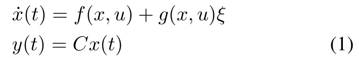
whereis the state vector,is the control input,is the measured output,is the fault signal,f(x,u) andg(x,u) are smooth vector field andis constant matrix. Consider a state observer with Luenberger like structure as follows:

The problem of state estimation and, consequently, residual generation is to design an observer, modeled by equations of the form (2), such that the residualewith dynamic equation(3) asymptotically converges to zero in absence of faultξ.So assumingg(x,u)̸= 0 the requirements of fundamental problem of residual generation (FPRG), i.e., the residualeonly is affected by faultξ, is satisfied.

The main challenge of designing observer (2) is to determine gain matrixLsuch that the convergence criterion of residualeis satisfied. The amount of mentioned gain and finite-time convergence are important attributes that should be considered. In [26], a procedure for optimal designing of a controller is presented.By utilizing that the method of optimal observer design for fault detection, is addressed as follows:

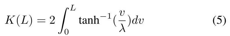
For the system (3) find an observer gainLsuch that the following finite-horizon performance function with its terminal cost is minimized.

To solve the constrained optimal nonlinear observer design,let

be the minimum cost of bringing the system (3) from initial conditione0to equilibrium point 0.

Definition 1 (Admissible observer gain):An observer gainLis defined to be admissible with respect to(6)on Ω,denoted bywithLcontinuous on Ω, if it stabilizes (3) forand foris finite.

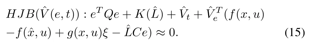
Under regularity assumptions, i.e.,considering (6) the HJB gives

whereandThisis a time-varying partial differential equation (PDE) withthat is the cost function for any givenand it is solved backward in time fromBy settingfor (6) we haveV(e(tf),tf)=ϕ(e(tf),tf).

IfLis the solution to the optimal observer design problem, then according to Bellman optimally principle [28], the optimal cost is given by

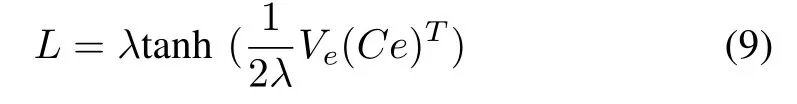
Optimal observer gain matrix,L, can be derived by solvingUsing (8) and (5), this equation can be written as

whereV(e,t)is the optimum value function.The time-varying observer gain matrix (??) represents constrained dynamic optimal observer for the nonlinear systems. The validity of an optimal observer design is expressed in the next theorem.

Theorem 1:Consider the nonlinear system (3) and performance function(6).Assume that there exists a functionV(e,t)as the solution of HJB equation (8). The observer (2) acts as an optimal residual generator that estimatexif no fault has occurredaddressing constraints with respect to terminal time and the observer gain. If a fault has occurredthe estimate ofxis such thatwhereϵis a positive constant.

Proof:Let us first study the case without the fault;we show thatLis a solution to the optimal observer design problem,i.e., the residuale(t) in system (3) converges to zero globally asymptotically, which can be proved by showingV(e,t), the solution of HJB equation (8), is a Lyapunov function.Clearly,V(e,t)>0 for∀e ̸= 0 andt ̸= 0 andV(0) = 0 also considering (8) we have

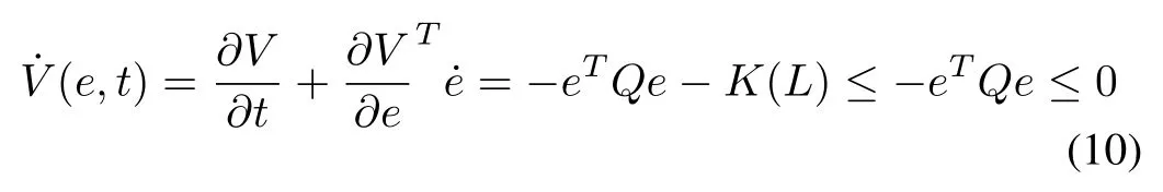
consequently, there exists a neighborhoodfor someϵ>0 such that ife(t) entersZ, then0.Bute(t)can not remain forever outsideZ.Otherwise0, for allt ≥0. Letsuch thatϵ. Therefore,we have

which contradicts the fact thatfor∀e ̸=0.

Let us now discuss the case when a fault has occurred.From(??) one can see that forthe time derivative of the estimation error is directly influenced by the fault. Since a fault is detectable, its occurrence causes a change in nominal behavior of system. So

Hence one can design a constrained optimal observer using proposed formulation for nonlinear systems with finite time horizon. An optimal observer can be designed by knowing exact solution of HJB equation, which is a difficult problem.In [22] utilizing a NN which is proposed in [26], the solution of HJB equation is approximated for calculating an observer gain related to an affine nonlinear system. In the next section,according to that NN, the approximation of value-functionVwhich is the solution of HJB equation is obtained.

B. NN Based HJB Solution

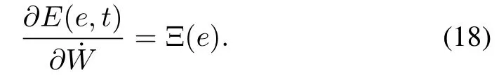
In this section, for finding approximate solution of HJB equation we use NN.In[29],it is shown that an online trained NN with time-varying weights can be used to approximate smooth time-varying functions on prescribed compact sets.Actually the approximate solution is used to find the observer gain. Therefore assuming thatV(e,t) is smooth and also uniformly continuous on a compact set Ω, one can use the following equation to approximateV(e,t) fort ∈[t0,tf] onΩ.

this is a NN with activation function=0. We have

and wheredenotes the NN weight andNis the number of hidden layer neurons,is the vector of activation function selected such thatandfor∀e ̸= 0 andt ̸= 0,is the vector of NN weights anddenotes the gradient of vectorwith respect toe. It is assumed thatNis large enough that there exist weightthat exactly satisfy the approximation att=tf. Without loss of generality, the setis selected to be independent and orthonormal [22]. The orthonormality of the setonimply that, for a real-valued function

whereis an inner product,andare continuous vector functions, and the series converge pointwise [30], i.e., for anyandΩ, one can chooseNsufficiently large to guarantee thatfor all time

Note thatin (8) is required, so the NN weights are selected to be time varying.Approximatingbyin the HJB equation (8) results in

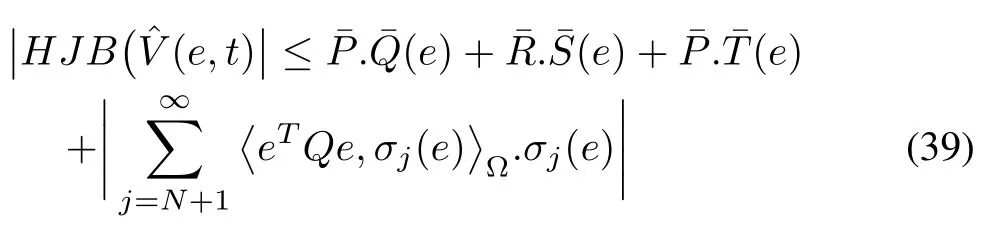
whereEis the approximation error. IfEis negligible, then(14) is similar to (8). Assuming the faultand coefficientsfor allNare uniformly bounded,the following lemma shows the existence of NN based HJB solution for optimal observer design using performance function (6).

Lemma 1:Givensuppose thatis inspace , and letandsatisfyHJB(V(e,t)) = 0 andV(e(tf),tf) =ϕ(e(tf),tf), thenuniformly on Ω asNincreases.

Proof:There is a theorem for the existence of NN based HJB solution for the optimal control problem in [26]. The existence of NN based HJB solution for optimal observer using modified performance functional can be proved on similar lines.See Appendix.

Since Lemma 1 shows the existence of NN based HJB solution, (14) can be written as

In the next theorem we prove that the nonlinear observer(2)is an optimum observer that estimates states in absence the fault and detects the fault when it occurs. It also proves the validity of the NN-HJB based observer design.Theorem 2:Consider the error dynamics (3) with the performance function (6). Assume that there exists a functionas the solution of HJB equation (14). Using this solution, if no fault has occurred observer gain matrixensures global asymptotic stability of system (3), i.e., errorasymptotically converges to zero. If a fault has occurred,whereϵis a positive constant.

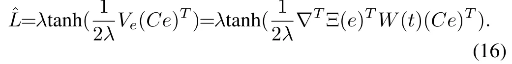
Proof: Using (12) and (15), we can find the approximate optimal observer gain matrix similarly as in (8) by following equation:withSo replacingwiththe system (3) remains globally asymptotically stable. Hence it can be proved thatthe solution of HJB equation (15) is a Lyapunov function.

From the above theorem we can say that an optimal observer with gain matrix (16) can be designed for a nonlinear system using HJB formulation. For calculating gain matrix, set of the NN weights is required. We describe this in the following.

The NN weights are selected to minimize approximation error in least square sense over a set of points sampled from a compact set Ω0inside the region of stability of the initial stabilizing control [31]. To find the least squares solution,the method of weighted residuals is used. This method was explored in [32] for optimal control problem based on HJB formulation. On similar lines, one can explore this method for observer design problem. The derivative of weightsWare determined by projecting the residual error ontoand setting the result to zerousing the inner product, i.e.,

Then (18) can be written as

Hence weight updating law can be obtained as

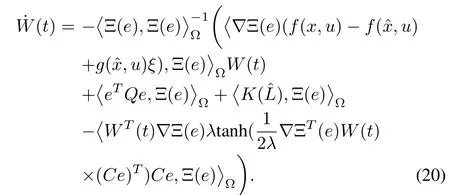
The NN weights can be determined by integrating (20)backwards in time using final conditionObserver gain(16) can be found using these weights.

Remark 1:So far state estimation and fault detection of nonlinear systems subject to a fault was studied.But when the system is subject to other unknown inputs like disturbances and more faults, the state estimation and FDI are more complicated. The recent statement is discussed in the next section more in detail.

III. STATE ESTIMATION AND FDI IN THE PRESENCE OF DISTURBANCES

A. The Residual Generation and its Affection of System Inputs

Consider systems modeled by equation of the form

The main problem is the design of an observer acting as a residual generator, modeled by equations of the form

Suppose the faultξj,1≤j ≤nξoccurs, rewrite (21) as

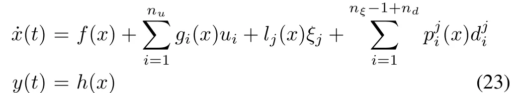
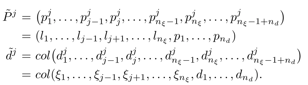
with

Assume the next filter is a residual generator with respect to the fault

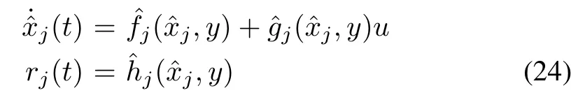
such that the responserjis affected by the inputξj, is decoupled from the input= 1,...,nξ −1 +ndand asymptotically converges to zero wheneverξjis identically zero, no matter whatuis.

The problem amounts to find a change of coordinates leading to a subsystem which is isolated from the disturbance, affected by the fault and observable. For the class of input affine nonlinear systems, a necessary condition for the nonlinear FPRG to be solvable was given by De Persis and Isidori in [19]. This result is based on differential geometric considerations and more precisely on the computation of the maximal observability codistribution which is locally spanned by exact differentials and is contained inUsing the same notations and terminology as in [19], the necessary condition for the existence of a solution to the local nonlinear FPRG is expressed by

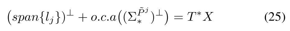
whereis cotangent space toX,is the minimal conditioned invariant distribution containingandis the maximal observability codistribution contained inin which the operatordenotes annihilator of the argument vector. On the basis of the mentioned codistribution, a change of coordinates is defined in[19] that leads to transform system (23) into the next form

Considering occurrence other faults instead ofξj, we can design a filter for the purpose of detecting multiple concurrent faultsξ1,...,ξnξ. According to (23) and filter (24), as a case of occurrence a fault, it is immediately shown that, if each filter detects its corresponding fault and is decoupled from the other, the bank of residual generators

solves the problem of detecting and isolating each individual fault signal

B. State Estimation and FDI

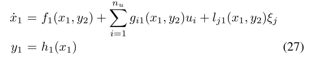
Referring to (1) we find that the system (27) lies in the form of these equations. So the fault signalξjexploiting the observer (2) can be detected.

Lemma 2:Consider system (21) and leth(x) =Cx,assume that condition(25)is satisfied and transformed system(27) as the first subsystem of (26) is given. Then for (27),addressing performance function (6), there exists an optimal nonlinear observer in the form of(2)with gain matrixL= ˆL,obtained by (16), that ensures global asymptotic stability of error dynamics in the form of (3) in the case ofξj=0. If the fault has occurred, i.e.,

Proof:Forh(x) =Cxand addressing condition (25), by following coordinate transformation of(26),thex1-subsystem can be rewritten as

This system lies in the form of (1). So considering (2)and (3), the related state observer and error dynamics can be written as

and

Using results of Lemma 1 and Theorem 2 in case ofξj=0 we havetherefore state vectorx1is estimated and consequently the occurrence of faultξjis detectable.

Remark 2:In order to detect and isolate other faults of the system (21), the procedure stated in this section can be repeated. By this way the bank of residual generator (28)that detects each fault and estimates related states will be determined.

IV. SIMULATION RESULTS

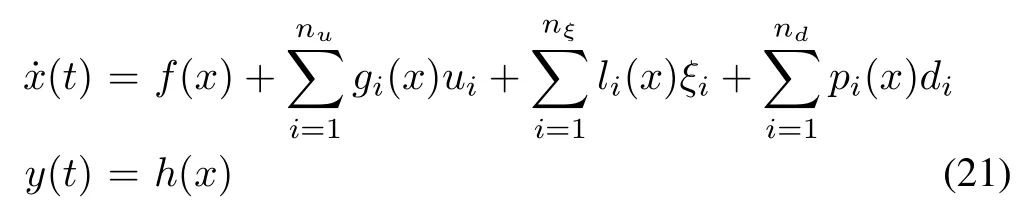
Consider a SLFJR system derived by a DC motor,see Fig.1,where the system nonlinearities come from the joint flexibility modeled as a stiffened torsional spring. A dynamical model for the robot can be described by the following equations[24].

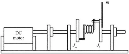
Fig.1. Schematic of an SLFJR electric drive system [24].

whereθmandωmare the motor position and angular velocity,respectively, andθlandωlrepresent those of the link. Variablesξ1andξ2denote plant and actuator fault signal anddrepresents an unknown disturbance input or any un-modelled dynamics.iais the armature current of the motor anduis the control input. The quantitiesθl,ia,ωm −ωlare available measurements of the system. The moment of inertia of the DC motor is denoted byJmwhile that of the controlled link is denoted byJl. Parameterhis the length of the link whilemrepresents its mass,BRstands for the viscous friction in the motor bearing,LmandRare the armature inductance and resistance, respectively.CtΦ is the product of torque coefficient and flux.klandk2both are positive constants andkτis the amplifier gain. The values of these parameters are given in Table I.

The aim of this study is to estimate the system state and detect and isolate the occurrence of faultsξ1andξ2in the armature current and excitation signal of the DC motor,respectively, in the presence of an unknown inputd.

Using relation (23) for faultξ1we have

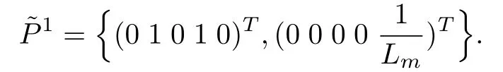
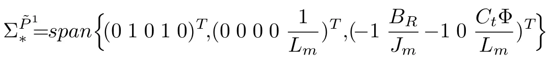
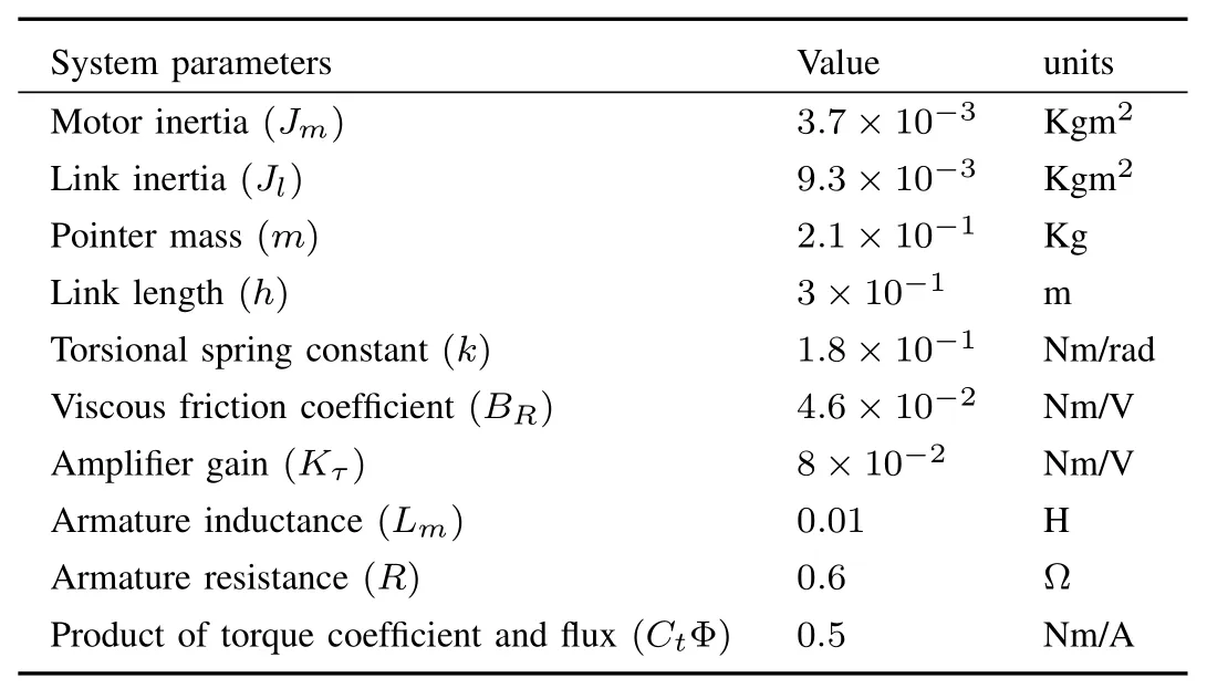
TABLE I VALUES OF SLFJR PARAMETERS

Referring to [19], the minimal conditioned invariant distribution containingcan be find as note thatis smooth, nonsingular and involutive for anyThen, its annihilator is locally spanned by exact differentials and can be expressed as follows:

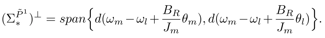
Also maximal observability codistribution which is locally spanned by exact differential can be computed as

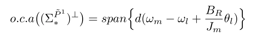
the coordinate transformation in the state space and output space induced byis given by

In the new coordinate, the system is rewritten as

On the other hand, for faultsξ2we have

following above steps forξ2one can obtain the next new coordinate system

where

Now utilizing the presented observer we want to detect the faults and estimate corresponding system states. Regard the first subsystem of (33), assumingy21=x21andy22=x22as independent inputs we have

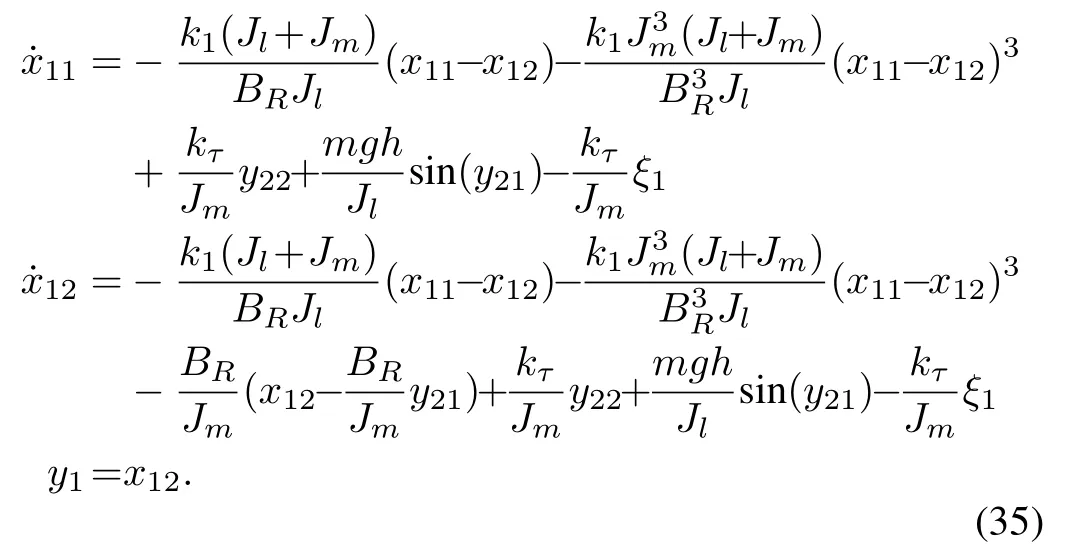
Using Lemma 2 we can calculateLand an observer in the form (30), the residual error for this system is

We have to find a nonlinear observer gainLthat minimize(6). Here we have selected

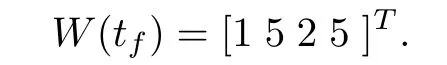
this is a NN with polynomial activation function.It is a power series NN of 4 activation functions containing powers up to 8th order of the error variable of the system. An appreciable change in the result is not observed if we use power series with order of 10 or more.It is also observed that for the power series up to 6th order, algorithm did not converge. So, design is carried out using the above mentioned. All the weights are determined by backward integrating equation (20). For this purpose we have selectedtf=30 s andW(tf) is as follows:

For the simulation, we have|L|≤5 andQ=1000.

For faultξ2by following the above procedure, regarding subsystem 1 of (34) and assumingy21=x21andy22=x22as independent inputs we can calculate that

and

The NN with polynomial activation function is

wheretf= 30 s,W(tf) = [10 1 3 1 5],|L| ≤11.5 andQ=2100.

For the simulation study, we assume that the system is initially at rest and fault free. At this time the observer is switched on with different initial condition than that of the system. At timet= 2 s the DC motor is excited byu= 7 per unit. As a result, the angular positions of the motor and the link, change to new non-zero steady-state values. Then att=7 s an abrupt fault occurs whereby the armature current is affected.The fault is fully cleared after 5 s.At timet=16 s an incipient fault occurs in the excitation system resulting in the gradual loss of the excitation signal and back to the previous situation over a period of 14 s. The applied faults are shown in Fig.2. It is assumed that throughout the simulation period the system is affected byd=0.1sin(0.1t).

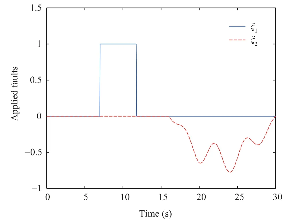
Fig.2. Applied faults to SLFJR electric drive system.

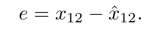
The results of simulation are shown in Figs.3−6. Fig.3 presents the residual erroreof system (35) and the observer gainLcorresponding to the faultξ1.It can be highlighted that the estimation erroreconverges towards zero when the faultξ1does not occur. When it appears att= 7 s, the residual signal shows an abnormal behavior of the system therefore the occurrence ofξ1is detectable. Fig.4 demonstrates the actual and estimated responses of the statesωm −ωl,θm,θlin which the estimation is result of an observer in the form(29) related to system (35).ωm −ωl,θmare obtained with the coordinate transformation mentioned in(33)and assuming availability ofθlas a measured output, also in Fig.4 (c),θlis obtained assuming availability ofωm −ωlas a measured output. Fig.5 presents the residual erroreof system (37) and the observer gainLcorresponding to the faultξ2. Here, likeξ1, the residual error converges toward zero when the fault does not occur and is affected by its occurrence att= 16 s.Finally considering coordinate transformation of system (34)and assuming availability ofia, estimation ofθlandθmin addition to their actual values are illustrated in Figs.6 (a) and(b). Also assuming availability ofθl,iais obtained, shown in Fig. 6 (c). It is clear from these figures that the observer is able to track the true state of the system.

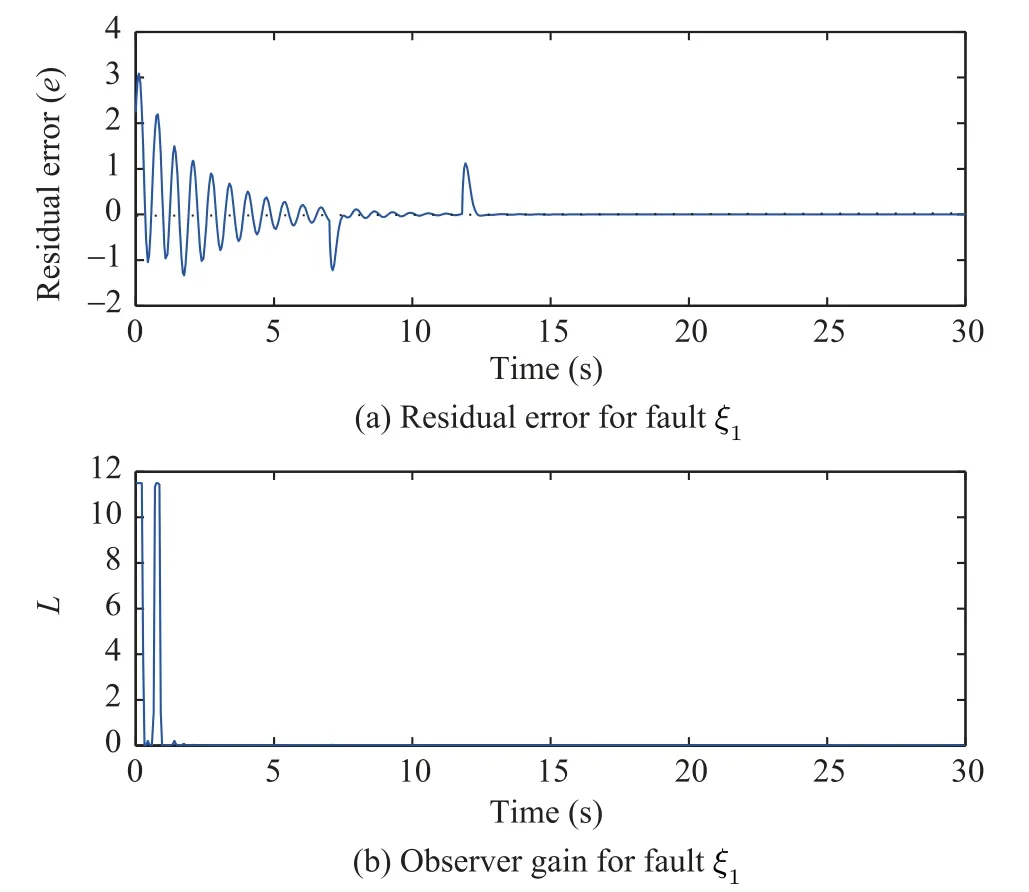
Fig.3. Residual error and observer gain for fault ξ1.

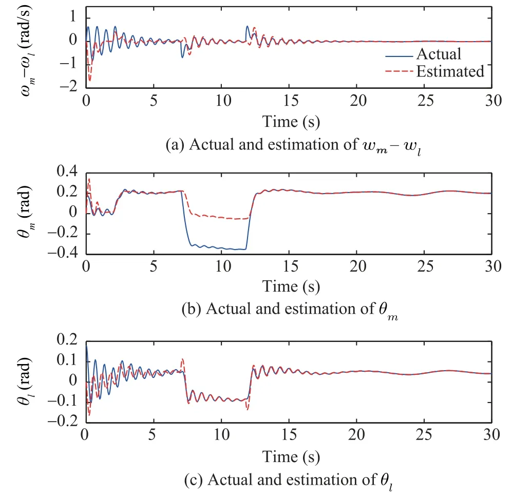
Fig.4. Actual and estimation of ωm − ωl,θm,θl.

As stated above, it has been considered here that an abrupt fault,ξ1, and an incipient fault,ξ2, occur in SLFJR electric drive system. According to the simulation results, it turns out that despite concurrent faults and unknown disturbance, the proposed approach is quite efficient in FDI. Figs.3 and 5,corresponding to the residual error and the observer gain ofξ1andξ2, respectively, reveal that each residual just is affected by corresponding fault and is not sensitive to the other or disturbanced. On the other hand, the estimated states related to the designed observer forξ1andξ2are shown in Figs.5 and 6, respectively. Since the observer is switched on with different initial condition than that of system, it is obvious that initially the estimated states differ from the actual values then converge on them. When a fault occurs the estimated states diverge from the actual ones. Detection and isolation of the fault actually is feasible by determining the mentioned divergence.

Fig.5. Residual error and observer gain for fault ξ2.

Fig.6. Actual and estimation of θl,θm,ia.

V. CONCLUSION

In this paper we presented an approach for state estimation and FDI in nonlinear systems in basis of optimal observer designing and differential geometry. At the beginning we brought out an optimal state estimator for wide class of nonlinear systems subject to an actuator or plant fault.Next we extended our work and considered a class of affine nonlinear systems which in addition to fault signals includes unknown disturbances. Utilizing a change of coordinates based on concept of observablility codistribution of differential geometry and under appropriate technical hypotheses, we transformed the system to a form in which there is a subsystem includes the fault signal and omits disturbances such that using the previous observer the subsystem states and its fault signal can be estimated and diagnosed, respectively. For other fault subject to the original system this procedure can be repeated.Finally,we used a simulation for a SLFJR electric drive model to illustrate the effectiveness of the presented approach.

In this study,it has been supposed that the nonlinear system is not subject to sensor fault. Also as another point, here the polynomial function(as a common activation function used for NN functions approximation)is considered for NN.Nonlinear observer design in the presence of sensor fault and considering another activation function like sigmoid function in NN, can be viewed as a further extension of this work.

APPENDIX

The hypothesis implies thatare inL2(Ω).Note that

Hence,

where

Therefore

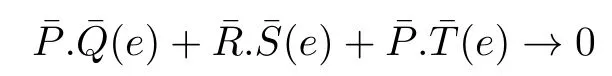
and