LIU Dong’ang, SUN Jian, and GUAN Changlong

Inversion of Evaporation and Water Vapor Transport Using HY-2 Multi-Sensor Data

LIU Dong’ang, SUN Jian*, and GUAN Changlong

Physical Oceanography Laboratory/CIMST, Ocean University of China and Qingdao National Laboratory for Marine Science and Technology, Qingdao 266100, China

HY-2 satellite is the first marine dynamic environment satellite of China. In this study, global evaporation and water vapor transport of the global sea surface are calculated on the basis of HY-2 multi-sensor data from April 1 to 30, 2014. The algorithm of evaporation and water vapor transport is discussed in detail, and results are compared with other reanalysis data. The sea surface temperature of HY-2 is in good agreement with the ARGO buoy data. Two clusters are shown in the scatter plot of HY-2 and OAFlux evaporation due to the uneven global distribution of evaporation. To improve the calculation accuracy, we compared the different parameterization schemes and adopted the method of calibrating HY-2 precipitation data by SSM/I and Global Precipitation Climatology Project (GPCP) data. In calculating the water vapor transport, the adjustment scheme is proposed to match the balance of the water cycle for data in the low latitudes.

HY-2 multi-sensor data; inversion; evaporation; water vapor transport; data calibration

1 Introduction

HY-2 satellite is the first marine dynamic environment satellite of China. It mainly carries a radar altimeter, a scanning microwave radiometer, a microwave scatterometer, and a correction microwave scatterometer. The primary goal is to monitor and survey the marine environment, including the sea wind, waves, currents, sea surface temperature, and other marine dynamic environment parameters. The satellite provides data on original sea wind, waves, currents, sea surface temperature, and other satellite-derived marine dynamic environments. These parameters are essential for global atmospheric and oceanic research. The interaction between the ocean and atmosphere is based on the flux of matter, energy, and momentum. Evaporation and water vapor transport play an important role in global water budget research and have a strong impact on these fluxes.

The most direct method to estimate evaporation is instrument measurement, namely, using the evaporating dish. However, this method is difficult to apply on an entire ocean. The aforementioned technical difficulty motivates the use of indirect calculation methods. Dalton proposed the evaporation formula based on aerodynamics (Dalton, 1802).Bowenratio-energybalancemethodproceededfrom energy balance formula (Bowen, 1926). Penman (1948) proposed the formula of free water surface evaporation using energy balance and aerodynamic concept. The eva- poration formula continues improvement and change (Table 1). Due to the rapid development of computer and space technology, a variety of parameterization schemes and models have been proposed, such as the European medium-range weather forecast model (Beljaars, 1995a, 1995b), Japan ocean flux remote sensing observation database products (Kubota and Mitsumori, 1997), and the atmospheric model of the National Center for Atmospheric Research (Collins, 2004) (Table 2).

For the study of the atmospheric water vapor, Fowle (1912) first proposed the estimation method of atmospheric precipitation derived from solar transmittance. Ben- ton and Estoque (1954) calculated the moisture content of the atmosphere and water vapor transport over the North American continent. The global water balance and northern hemisphere atmospheric water vapor transport was studied in the 1960s (Starr and Peixoto, 1964). Water vapor transport and its relationship with evaporation and precipitation were further studied (Peixoto, 1973; Peixoto, 1982). Based on previous research, a more complex eigenvalue tracking algorithm for water vapor transport is proposed. (Hilburn, 2009).

Besides the conventional measurements and numerical models (Roads, 1994; Gutowski, 1997; Roads, 2002), the satellite shows the potential of estimating the evaporation and water vapor transport in the ocean. Satellites can provide large-scale and long-term global atmospheric and oceanic data, and combined with inversion algorithm, evaporation and water vapor transport can be represented more accurately. New methods based on satellite data are also being studied continuously. Estimation of evaporation based on MODIS satellite data was continuously studied (Zhao, 2005; Cleugh, 2007). Dobler(2011) compared various semi-empirical methods to determine potential and actual evaporation from satellite data. Water vapor transport over the ocean was analyzed using satellite data (Sohn, 2002; Sohn, 2004).

Based on the preceding methods, this paper uses the original HY-2 multi-sensor data to calculate the evaporation and water vapor transport, and part of the original data is calibrated through other reanalysis data. Section 2 describes the original HY-2 data and reanalysis data from the other agencies. In Section 3, the method to estimate evaporation and water vapor transport are described. The results of evaporation and water vapor transport are presented in Section 4. We summarize and discuss the major findings in Section 5.

Table 1 Calculation formula of evaporation in different periods

Table 2 Formula and parameterization scheme used by different agencies

2 Data

HY-2 multi-sensor data mainly contains sea surface tem- perature (SST), sea surface wind (SSW), and sea surface precipitation. The domain of interest is restricted to 180˚E–180˚W and 80˚N–80˚S. The spatial resolution of data is regular 0.03˚×0.03˚ longitude-latitude grid. The accuracy of SST (SSW) is approximately 1.0K (2ms−1). The HY-2 SST and buoy SST provided by China Argo real-time data center are fitted to determine the accuracy of HY-2 data, as shown in Fig.1, and the linear fit coefficient is 1.038. ARGO data are the global gridded data (BOA_Argo) set with a spatial resolution of 1˚ (Lu, 2019). The dataset is produced based on refined Barnes successive corrections by adopting flexible response functions based on a series of error analyses to minimize errors induced by nonuniform spatial distribution of Argo observations (Li, 2017). Although the SST comes from different measurement methods, the HY-2 data are consistent with the buoy data provided by ARGO, which indicates that the sea surface temperature provided by HY-2 is credible.

The following reanalysis data are used in the investigations below: 1) mean daily air temperature at sigma level 995(NationalCentersforEnvironmentalPrediction (NCEP)), 2) mean daily pressure at the surface (NCEP), and 3) daily relative humidity at sigma level 995 (NCEP). The observational datasets are 1) average monthly rate of precipitation, which is provided by a remote sensing system; and 2) average monthly rate of precipitation, which is provided by the Global Precipitation Climatology Project (GPCP). The details of the data are shown in Table 3.

HY-2 data is a non-grid provided by satellite microwave radiometer and scanning scatterometer. Therefore, before inversion calculation, the data need to be re-gridded as monthly mean gridded data. The SST provided by HY-2 has been corrected by the National Ocean Satellite Application Center, but it still has abnormal values in some high latitudes. Therefore, the abnormal values are eliminated in the process of calculating the monthly average. To insert the original data to the regular grid, we use the natural neighbor interpolation method (Sibson, 1981), and the equation is as follows:

Fig.1 Liner fitting of HY-2-SST (developed using the original data) and Argo-SST.

Table 3 Introduction of data provided by other agencies

where(,) is the estimated value at (,), andwis the weight corresponding to theth known data(x,y) at (x,y). The weight,w, is calculated by finding how much of each of the surrounding areas is ‘stolen’ when inserting (,) into the tessellation.

3 Method

3.1 Inversion of Evaporation

Evaporation (E) is a type of vaporization that occurs on the surface of a liquid as it changes into the gas phase. According to the bulk aerodynamic method (Thornthwaite and Holzman, 1939), evaporation can be expressed as

whereairis the density of air,Cis the exchange coefficient for water vapor at height,Uis the wind speed at height,qis the specific humidity at the sea surface, andqis the specific humidity at height. The bulk formula has been found from field experiments where the total evaporationhas been measured directly together with mean values of specific humidity and wind speed at height. The heightis 15m. Fig.2 shows the detailed steps of data processing and calculation.

The density of air and specific humidity are calculated by the Goff-Gratch equation (Goff and Gratch, 1946). Wet air density can be represented as

whereρairis the density of dry air,is relative humidity,Eis saturated vapor pressure, andis air pressure. Dry air density is as follows:

whereis the air temperature.,, andare provided by NCEP data according to the Goff-Gratch formulation (Pol, 1998),

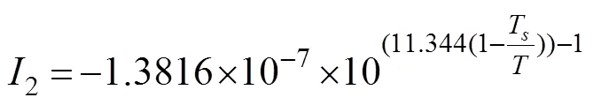
whereTis the steam-point temperature.

According to the relationship of specific humidity and mixing ratio, the sea surface saturation specific humidity and 15m specific humidity can be calculated by the following formula:

In the ocean surface, water vapor at the air-sea interface can be assumed to be saturated. The saturated mixing ratio can be calculated as follows:

whereFis the correction factor for the departure of the mixture of air and water vapor from ideal gas laws, and it is given by

whereis the absolute dew point temperature. The surface saturated specific humidity can be obtained by Eqs. (9) and (10). In particular, the coefficient of 0.981 is used to adjust the effect of salinity (Hillburn, 2009). According to the definition of relative humidity,

whereqandqare specific humidity at heightand saturated specific humidity.qcan be calculated by RH (provided by NCEP) and saturated humidity.

The parameterChas an important influence on evaporation. The parameterization schemes used by different institutions vary widely. Through the measurement experiment,Cis close to a constant. According to the experiments of Surface of the Oceans, Fluxes, and Interaction with the Atmosphere (SOFIA) and Structure des Echanges Mer-Atmosphere, Properties des Heterogeneites Oceaniques Recherche Experimentale (SEMAPHORE) (Dupuis, 1997),

However, on a global scale, consideringCas a constant will lead to large errors. According to the relevant specific humidity and evaporation formula, the relationship betweenCand water vapor roughness can be derived as follows:

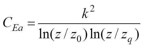
where0is the momentum roughness andzis the water vapor momentum roughness. Roughness is a function of friction velocity (*) based on the European center parameterized scheme.

The sea-air interface wind stress depends on the SSW speed, atmosphere stratification stability, and sea state. Based on the Monin-Obukhov similarity theory, the surface wind speed profile can be expressed as

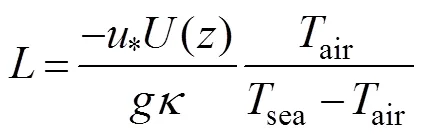
whereis the Karman constant, which is usually 0.4, andis the Monin-Obukhov length (Foken, 2006), which can be expressed as

The stability function(/)can be determined by Businger-Dyer expression (Dyer and Hicks, 1970; Businger, 1971). For the stable atmospheric stratification (>0),

Then, for the unstable atmospheric stratification (<0),

Ccan be obtained by the iterative approach when the wind speed, air temperature, and SST are determined. Thus, through these parameters, the evaporationcan be finally obtained.

3.2 Inversion of Water Vapor Transport

Water vapor transport represents a certain amount of water vapor that flows through a unit area in unit time. Fig.3 shows the detailed steps for calculating the water vapor transport, on which precipitation (P) has an important influence. As the precipitation rate data are not initially corrected when generating the original data, the accuracy of original precipitation rate data is worse. Precipitation data need to be calibrated because the microwave remote sensing is insensitive to solid-phase precipitation in the atmosphere and HY-2 precipitation data in the mid-latitude regions involve a larger amount of errors.

The GPCP conforms well to the observed data especially in high latitudes. The Special Sensor Microwave Imager (SSM/I) has good time matching to GPCP. Meanwhile, the SSM/I precipitation rate data in the mid-latitudes also has a high resolution and good accuracy. Thus, the original precipitation rate can be calibrated by these datasets. In the following three cases, the precipitation rate is calibrated as follows: A) The data point is erroneous or missing. B) The data point has a large error. C) Solid-phase precipitation correction is conducted. We set the following adjustment factor:

Whenvalue is less than 30%, we do not process the value of the data point. For the correction of solid-phase precipitation in high latitudes, we use the following method. The condition for calibration is the data point value(,) that meets the following condition:

Using the calibrated precipitation and evaporation, we can begin to calculate the water vapor transport. According to the water balance relationship on monthly mean scale, water vapor transport divergence is shown as follows (Peixoto and Oort, 1992):

where is the water vapor transport that is mainly calculatedusingthefollowingformulainmeteorology(Peixoto, 1973):

This algorithm in the smaller area is accurate. However, in the global scale, this algorithm becomes biased. To obtain realistic estimates of divergence, we have to adjust the transport vectors until the divergence equals−. This technique was based on previous work by Hilburn(2003). Applying Helmholtz theorem (Holton and Hakim, 2012), the method is as follows:

For the HY-2 product, we used Dirichlet boundary conditions, and to fill the default value of the land, we used values of−=(527−806)/8766mmh−1(Wentz, 2007). Notably, in the calculation of the gradient, divergence and Laplacian operator are needed in the earth system.

4 Results

Fig.4 shows the global inversion evaporation using HY-2 multi-sensor data in April 2014. The spatial resolution of the evaporation is 0.1˚. The global evaporation distribution varies with latitude. The evaporation in low- and middle-latitude areas is significantly higher than that in high-latitude areas. The large values of evaporation areas, which are generally greater than 0.3mmh−1, are located around the equator from 30˚N to 30˚S. The small values, which are generally less than 0.1mmh−1, appear in the north and south poles and other high latitudes. This distribution is consistent with the global energy distribution. In the equatorial region, the value is small, which is due to the perennial rain near the equator. Furthermore, solar radiation extinction effect caused by clouds is strong, and the doldrums occur in the equator with weak convection. Therefore, the equatorial evaporation is weak.

Fig.5 shows the scatter plot of HY-2 evaporation and OAFlux evaporation. Compared with the reanalysis data, OAFlux data, the distribution of HY-2 evaporation shows a similar pattern (not shown). However, the result of HY-2 is slightly higher than that of OAFlux. The reason for this discrepancy shows the possibility that the algorithms are different. Two clusters exist, which are approximately 0.05mmh−1and 0.15mmh−1. The global SST is evenly distributed from low to high, while evaporation is mainly concentrated in two high-value regions. This condition also shows that evaporation is unevenly distributed around the world, being high in the subtropical high-pressure belt and low in other regions.

Air density, specific humidity, and exchange coefficient have crucial impacts on evaporation. Fig.6 shows the global air-density distribution. According to the calculation formula of air density, the increasing humidity of the air is related to the decreasing air density. In the middle and low latitudes, due to the high evaporation and specific humidity, the air contains a larger amount of water vapor. However, the density of water vapor is less than that of dry air, so the wet air density in these regions is less than that in high latitudes. This distribution trend corresponds to the distribution of the specific humidity. Fig.7 is the global specific humidity distribution. The left and right sides are the sea saturation specific humidity and the specific humidity at 10m. Saturation specific humidity of the sea surface and 10m specific humidity has obvious discrepancy which is contributed by the evaporation of water and the transport to other areas.

Fig.4 Inversion of the global gridded monthly average evaporation (mmh−1).

Fig.5 Scatter plot of HY-2 and OAFlux evaporation.

Fig.6 Global air-density distribution (kgm−3).

Fig.7 Global specific humidity distribution, the left side is the sea saturation specific humidity and the right side is the specific humidity at 10m (gkg−1).

Cis the exchange coefficient for water vapor. Its global distribution is shown in Fig.8.Cis not a constant and it changes with the air-sea condition. Substantial research has shown that it varies with the wind speed. Chas a complicated relationship with wind speed according to the observed data. With low (high) wind speed,Cand wind speed have a negative (positive) correlation, and gradually tend to be invariable. However, due to the lack of observed data, the change law of0andz, which are the essential parameters to calculateC, is still under debate. If the empirical values of0andzare invariable under different atmospheric and oceanic conditions, thenCincreases with the wind speed. Another view is that0andzreduce along with the wind speed growth; in this case,Cis invariable (Large and Pond, 1982; Decosmo, 1996). The calculation method for wind speed used in this study is derived from the parameterization scheme of the European center. Fig.8 shows the global exchange coefficient for water vapor distribution, and Fig.9 presents the fitting results ofCand wind speed. When the wind speed is less than 4ms−1,Creduces along with the wind speed. When the wind speed is stronger than 4ms−1,Cincreases with the wind speed. At present, due to the insufficient calculation method of C, different calculation results have various effects on the evaporation rate. Therefore, improving the accuracy of Ccan effectively improve the accuracy of the evaporation calculation.

Fig.10 shows the adjusted HY-2 precipitation rate. The maximum precipitation area is located at the equator and decreases with increasing latitude. The western equatorial Pacific, West African monsoon precipitation area, northern regions of South America, and southeastern China to Japan area are the maximum precipitation areas. However, less precipitation is observed in most parts of northern Africa, the Middle East and Central Asia, western Australia, the Pacific northwest and southeast of the Atlantic, and southeast of the Indian Ocean.

The zonal mean of evaporation is the bimodal structure. The reason is that two subtropical high-pressure belts exist, which have particularly large evaporation. The zonal mean of precipitation is the unimodal structure because precipitation is mainly concentrated in the equator, as shown in Fig.11. When the factors of land are removed, the area of evaporation and precipitation enclosed by theaxis should be roughly equal. The peak of evaporation is the area 15˚ north and south of the equator, and the peak of precipitation is near the equator, which is consistent with the global distribution. Fig.12 shows the water vapor transport divergence, which represents the relationship between evaporation and precipitation in this region. The blue part represents the area where precipitation is greater than evaporation, and the red part is reversed.

Fig.8 Global exchange coefficient for water vapor distribution (dimensionless parameter).

Fig.9 Fitting results of CE and wind speed.

Fig.10 Adjusted HY-2 precipitation rate based on SSM/I and GPCP data (mmh−1).

Fig.11 Zonal mean evaporation (blue solid line, mmh−1), precipitation (blue dotted line, mmh−1), and water vapor transport (gskg−1).

Fig.12 Water vapor transport divergence; blue part represents the area where precipitation is greater than evaporation, and the red part represents the vice versa (mmh−1).

Fig.13 shows the global water vapor transport without adjustment, of which distribution presents a significant north–south asymmetry. North Pacific water vapor transport is stronger than that in the South Pacific. The Indian Ocean region, northeastern Australia, and northeast South America also show strong water vapor transport. In high latitudes, water vapor transmission is weak. It has a good corresponding relation with precipitation. Due to the impact of the monsoon, a large amount of water vapor is transported to Southeast Asia, northern South America, and central Africa. Fig.14 shows the global water vapor transport with adjustment, which is slightly higher than that without adjustment in Fig.13. Fig.15 shows the water vapor transport difference value between adjustment and no adjustment, and indicates that the divergence adjustment is crucial to water vapor transport, especially in the mid-latitude region, which is the area where water vapor is most concentrated.

Fig.13 Water vapor transport without the adjustment (gskg−1).

Fig.14 Water vapor transport with the adjustment (gskg−1).

Fig.15 Water vapor transport difference value between adjustment and no adjustment (gskg−1).

5 Discussion and Summary

The detailed inversion methods by using HY-2 data of evaporation, precipitation, and water vapor transport are introduced in this paper. The reality of global evaporation and water vapor transport are shown, and their global distribution is discussed. Since the data on HY-2 are enormous and complex, the results are based on the limited data in April 2014. The seasonal and annual results will be further studied in the future to evaluate the accuracy of the algorithm.

We also compared the sea surface temperatures of HY-2 and ARGO, and found that SST distributed uniformly from low to high temperature, and the satellite and ARGO data have a good consistency. The linear fitting coefficient of the HY-2 SST data and ARGO data is 1.038. Comparing the evaporation of HY-2 with that of OAFLUX, we find that the evaporation values are mainly concentrated in two parts. The reason is that the evaporation in the subtropical high-pressure belt is significantly larger than that in other regions, and the values in other regions are very close. The HY-2 original precipitation data is calibrated by SSM/I and GPCP precipitation data due to the poor accuracy of the original data. In the process of water vapor transport calculation, we apply a new method to adjust the results of the traditional calculation formula. The new result for the accuracy of the water vapor transport in low and middle latitudes has a significant improvement.

To enhance the accuracy of the results, the following methods can be applied:

1) Using the high-resolution data of other agencies, which is the most effective way to improve the accuracy of the results.

2) Trying to use different parameterization schemes and parameters. The parameterization schemes and algorithms used in this study may not be the most accurate on a global scale. Therefore, using different methods may bring more accurate results.

3) Using various methods of water vapor transport adjustment. The adjustment method used in this study has an important effect on water vapor transport in the low- and middle-latitude regions. However, no significant correction occurs in the middle and high latitudes. Therefore, using different adjustment methods for different regions will improve the accuracy of the results.

Acknowledgements

The authors appreciate the financial support from the National Natural Science Foundation of China (No. 41976017), the Ministry of Science and Technology of China (No. 2016YFC1401405), and the National Natural Science Foundation of China (No. U1406401).

Beljaars, A. C. M., 1995a. The parametrization of surface fluxes in large-scale models under free convection.,121 (522): 255-270.

Beljaars, A. C. M., 1995b. The impact of some aspects of the boundary layer scheme in the ECMWF model. In:. Reading, 125-161.

Benton, G. S., and Estoque, M. A., 1954. Water-vapor transfer over the North American continent.,11 (6): 462-477.

Bowen, I. S., 1926. The ratio of heat losses by conduction and by evaporation from any water surface.,27 (6): 779.

Businger, J. A., Wyngaard, J. C., Izumi, Y., and Bradley, E. F., 1971. Flux-profile relationships in the atmospheric surface layer.,28 (2): 181-189.

Cleugh, H. A., Leuning, R., Mu, Q., and Running, S. W., 2007. Regional evaporation estimates from flux tower and modis satellite data., 106 (3): 285-304.

Collins, W. D., Rasch, P. J., Boville, B. A., Hack, J. J., McCaa, J. R., Williamson, D. L., Kiehl, J. T., and Briegleb, B., 2004.. NCAR Technical Note, National Center for Atmospheric Research, Boulder, Colorado, 214pp.

Dalton, J., 1802. Experimental essays on the constitution of mixed gases; on the force of steam or vapor from water and other liquids in different temperatures, both in a Torricellian vacuum and in air; on evaporation and on the expansion of gases by heat., 5 (2): 535-602.

DeCosmo, J., Katsaros, K. B., Smith, S. D., Anderson, R. J., Oost, W. A., Bumke, K., and Chadwick, H., 1996. Air-sea exchange of water vapor and sensible heat: The humidity exchange over the sea (HEXOS) results.,101 (C5): 12001-12016.

Dobler, A., Müller, R., and Ahrens, B., 2011. Development and evaluation of a simple method to estimate evaporation from satellite data., 20 (6): 615-623.

Dupuis, H., Taylor, P. K., Weill, A., and Katsaros, K., 1997. Inertial dissipation method applied to derive turbulent fluxes over the ocean during the surface of the ocean, fluxes and interactions with the atmosphere/atlantic stratocumulus transition experiment (SOFIA/ASTEX) and structure des echanges mer-atmosphere, proprietes des heterogeneites oceaniques: recherche experimentale (SEMAPHORE) experiments with low to moderate wind speeds.,102 (C9): 21115-21129.

Dyer, A. J., and Hicks, B. B., 1970. Flux-gradient relationships in the constant flux layer., 96(410): 715-721.

Foken, T., 2006. 50 years of the Monin-Obukhov similarity theory.,119 (3): 431-447.

Fowle, F. E., 1912. The spectroscopic determination of aqueous vapor.,35: 149.

Goff, J. A., and Gratch, S., 1946. Low-pressure properties of water from −160 to 212˚F.. New York, 95-122.

Gutowski, W. J. J., Chen, Y., and Ötles, Z., 1997, Atmospheric water vapor transport in NCEP-NCAR reanalyses: Comparison with river discharge in the central united states., 78 (9): 1957-1969.

Harbeck Jr., G. E., Kohler, M. A., and Koberg, G. E., 1958.Geological Survey Professional, U. S. Government Printing Office, Washington D. C., Paper 298, 100pp.

Hilburn, K. A., 2009. The passive microwave water cycle product.. Remote Sensing Systems, Santa Rosa, CA,30pp.

Hilburn, K. A., Bourassa, M. A., and O’Brien, J. J., 2003. Development of scatterometer-derived surface pressures for the Southern Ocean.,108 (C7): 3244, DOI: 10.1029/2003JC001772.

Holton, J. R., and Hakim, G. J., 2012.. Academic Press, Massachusetts, 67pp.

Kubota, M., and Mitsumori, S., 1997. Sensible heat flux estimated by using satellite data over the North Pacific.,8: 127-136.

Kuzmin, P. O., 1957. Hydrophysical investigations of land waters.,3: 468-478.

Large, W. G., and Pond, S., 1982. Sensible and latent heat flux measurements over the ocean.,12 (5): 464-482.

Li, H., Xu, F., Zhou, W., Wang, D., Wright, J. S., Liu, Z., and Lin, Y., 2017. Development of a global gridded argo data set with barnes successive corrections., 122 (2): 866-889.

Lu, S. L., Liu, Z. H., Li, H., Li, Z. Q., Wu, X. F., Sun, C. H., and Xu, J. P., 2019.. China Argo Real-Time Data Center, 26pp.

Peixoto, J. P., 1973.. Secretariat of the World Meteorological Organization, Geneva, 81pp.

Peixoto, J. P., and Oort, A. H., 1992.. American Institute of Physics.New York, 520pp.

Peixoto, J. P., De Almeida, M., Rosen, R. D., and Salstein, D. A., 1982. Atmospheric moisture transport and the water balance of the Mediterranean Sea.,18 (1): 83-90.

Penman, H. L., 1948. Natural evaporation from open water, bare soil and grass., 193 (1032): 120-145.

Pol, S. L. C., Ruf, C. S., and Keihm, S. J., 1998. Improved 20- to 32-GHz atmospheric absorption model.,33 (5): 1319-1333.

Press, W., Teukolsky, S., Vetterling, W., and Flannery, B., 1992.. Cambridge University Press, Cambridge, 933pp.

Roads, J. O., Chen, S. C., Guetter, A. K., and Georgakakos, K. P., 1994. Large-scale aspects of the united states hydrologic cycle., 75 (9): 1589-1610.

Roads, J. O., Kanamitsu, M., and Stewart, R., 2002. CSE water and energy budgets in the NCEP DOE reanalysis II., 3 (3): 227-248.

Sibson, R., 1981. A brief description of natural neighbour interpolation.,21: 21-36.

Sohn, B. J., Smith, E. A., Robertson, F. R., and Park, S. C., 2004. Derived over-ocean water vapor transports from satellite-retrieved E-P datasets., 17 (6): 1352-1365.

Sohn, B., 2002. Use of satellite-derived rainfall data for diagnosing water vapor transport over the global oceans. In:Houston, Texas, No. 2346.

Starr, V. P., and Peixoto, J. P., 1964. The hemispheric eddy flux of water vapor and its implications for the mechanics of the general circulation.,14(2): 111-130.

Thornthwaite, C. W., and Holzman, B., 1939. The determination of evaporation from land and water surfaces., 67 (1): 4-11.

Wentz, F. J., Ricciardulli, L., Hilburn, K., and Mears, C., 2007. How much more rain will global warming bring?,317(5835): 233-235.

Zhao, M., Heinsch, F. A., Nemani, R. R., and Running, S. W., 2005. Improvements of the MODIS terrestrial gross and net primary production global data set., 95 (2): 164-176.

April 8, 2019;

June 21, 2019;

September 29, 2019

© Ocean University of China, Science Press and Springer-Verlag GmbH Germany 2020

. Tel: 0086-532-66786228

E-mail: sunjian77@ouc.edu.cn

(Edited by Xie Jun)